Dupilumab in children and adolescents (Kovalenko 2021)
Source:vignettes/articles/Kovalenko_2021_dupilumab.Rmd
Kovalenko_2021_dupilumab.RmdModel and source
- Citation: Kovalenko P, Kamal MA, Davis JD, Huniti N, Xu C, Bansal A, Shumel B, DiCioccio AT. Base and Covariate Population Pharmacokinetic Analyses of Dupilumab in Adolescents and Children >=6 to <12 Years of Age Using Phase 3 Data. Clinical Pharmacology in Drug Development. 2021;10(11):1345-1357. doi:10.1002/cpdd.986
- Article: Clin Pharmacol Drug Dev. 2021;10(11):1345-1357 (open access via PMC8597115)
- Supplement: Supplementary Tables 1-5 (between-subject variability, residual error and bootstrap intervals), distributed with the article.
Kovalenko 2021 applied the adult dupilumab model of Kovalenko 2020
(readModelDb("Kovalenko_2020_dupilumab_covariate")) without
structural change to two phase 3 pediatric atopic-dermatitis trials, and
analysed the two age groups separately. Each age group has a primary
base model (body weight on central volume only) and a primary covariate
model:
| Model | Age group | Covariates |
|---|---|---|
Kovalenko_2021_dupilumab_children_base |
6 to <12 years | WT on Vc |
Kovalenko_2021_dupilumab_children_covariate |
6 to <12 years | WT, ALB on Vc; EASI on ke |
Kovalenko_2021_dupilumab_adolescent_base |
12 to <18 years | WT on Vc |
Kovalenko_2021_dupilumab_adolescent_covariate |
12 to <18 years | WT on Vc; BMI, EASI on ke |
The model is a two-compartment model parameterised in rate constants (Vc, ke, kcp, kpc) with parallel linear and Michaelis-Menten (Vm, Km) elimination from the central compartment. Subcutaneous doses pass through three transit compartments (mean transit time MTT) into an absorption depot drained at ka, with bioavailability F (Figure 1). Only Vc, ke and (except in the children covariate model) Vm were estimated; the remaining structural parameters were fixed to the adult values, except ka in children, which was estimated on the semisparse phase 2a R668-AD-1412 data and then fixed.
The sensitivity analyses parameterised in clearance (Tables 3 and 4, Supplementary Tables 4 and 5) are not packaged; the paper presents them as robustness checks of the rate-parameterised primary models.
Population
- Children 6 to <12 years (R668-AD-1652, LIBERTY AD PEDS, NCT03345914): severe atopic dermatitis with concomitant topical corticosteroids; 239 of 241 children on active treatment and 925 of 1173 samples entered the primary analysis. Mean (SD) age 8.5 (1.7) years, weight 31.6 (10.2) kg, 49.8% male. Regimens: 100 mg every 2 weeks (q2w) for <30 kg (n = 63), 200 mg q2w for >=30 kg (n = 59), or 300 mg every 4 weeks (q4w) (n = 119).
- Adolescents 12 to <18 years (R668-AD-1526, LIBERTY AD ADOL, NCT03054428): moderate-to-severe atopic dermatitis, dupilumab monotherapy; 162 of 165 adolescents on active treatment and 827 of 1006 samples. Mean (SD) age 14.4 (1.59) years, weight 65.3 (22.0) kg, 56.7% male. Regimens: 200 mg q2w for <60 kg (n = 43), 300 mg q2w for >=60 kg (n = 39), or 300 mg q4w (n = 82).
In both studies PK samples were collected on days 1, 29, 57 and 113
and at the end of treatment (Methods). The same information is available
programmatically via
readModelDb("Kovalenko_2021_dupilumab_children_base")()$population
(and likewise for the other three models).
Source trace
Every ini() value carries an in-file comment naming its
source row. The table collects them. Values are identical in Table 1 /
Table 2 of the article and in Supplementary Tables 2 / 3, which add the
between-subject variability and residual error.
| Parameter | Children base | Children covariate | Adolescent base | Adolescent covariate | Source |
|---|---|---|---|---|---|
| Vc (L, at 75 kg) | 2.22 | 2.18 | 2.54 | 2.47 | Table 1 / Table 2 |
| ke (1/d) | 0.0444 | 0.0446 | 0.0508 | 0.0520 | Table 1 / Table 2 |
| Vm (mg/L/d) | 1.64 (estimated) | 1.64 (fixed) | 1.46 | 1.43 | Table 1 / Table 2 and footnotes; Methods |
| Km (mg/L) | 0.01 (fixed) | 0.01 (fixed) | 0.01 (fixed) | 0.01 (fixed) | Table 1 / Table 2 |
| kcp (1/d) | 0.211 (fixed) | 0.211 (fixed) | 0.211 (fixed) | 0.211 (fixed) | Table 1 / Table 2 |
| kpc (1/d) | 0.310 (fixed) | 0.310 (fixed) | 0.310 (fixed) | 0.310 (fixed) | Table 1 / Table 2 |
| ka (1/d) | 0.641 (fixed) | 0.641 (fixed) | 0.306 (fixed) | 0.306 (fixed) | Table 1 / Table 2 |
| MTT (d) | 0.105 (fixed) | 0.105 (fixed) | 0.105 (fixed) | 0.105 (fixed) | Table 1 / Table 2 |
| F | 0.642 (fixed) | 0.642 (fixed) | 0.642 (fixed) | 0.642 (fixed) | Table 1 / Table 2 |
| Vc ~ weight | 0.864 | 0.849 | 0.853 | 0.755 | Table 1 / Table 2 |
| Vc ~ albumin | – | -0.525 | – | – | Table 2 |
| ke ~ BMI | – | – | – | 0.357 | Table 2 |
| ke ~ EASI | – | 0.169 | – | 0.356 | Table 2 |
| SD(ln Vc) | 0.305 | 0.291 | 0.141 | 0.140 | Supp. Table 2 / 3 |
| SD(ln ke) | 0.409 | 0.417 | 0.335 | 0.304 | Supp. Table 2 / 3 |
| Corr(ln ke, ln Vc) | -0.871 | -0.883 | -0.407 | -0.529 | Supp. Table 2 / 3 |
| Proportional SD | 13.2% | 13.1% | 9.90% | 9.94% | Supp. Table 2 / 3 |
| Additive SD (mg/L) | 0.03 (fixed) | 0.03 (fixed) | 2.41 | 2.36 | Supp. Table 2 / 3 |
| Continuous covariate form | Y * (cov / central value)^theta |
Methods, first formula | |||
| Weight central value | 75 kg | Methods | |||
| Structure | 2-cmt, rates, linear + MM elimination, 3 transit compartments | Methods; Figure 1 |
Checks against values printed in the paper
Derived parameters and beta half-life
Supplementary Tables 2 and 3 print CL = Vc * ke, Q = Vc * kcp and Vp = Vc * kcp / kpc for every model, and the Discussion quotes the beta half-life (the slower disposition half-life of the linear two-compartment system, a function of ke, kcp and kpc only) as 27.1 days in children and 23.4 days in adolescents. These are exact functions of the packaged typical values, so they are checked to printing precision.
models <- c(
  children_base        = "Kovalenko_2021_dupilumab_children_base",
  children_covariate   = "Kovalenko_2021_dupilumab_children_covariate",
  adolescent_base      = "Kovalenko_2021_dupilumab_adolescent_base",
  adolescent_covariate = "Kovalenko_2021_dupilumab_adolescent_covariate"
)

beta_half_life <- function(ke, kcp, kpc) {
  s <- ke + kcp + kpc
  log(2) / ((s - sqrt(s^2 - 4 * ke * kpc)) / 2)
}

derived <- bind_rows(lapply(names(models), function(nm) {
  th <- rxode2::rxode2(readModelDb(models[[nm]]))$theta
  vc <- exp(th[["lvc"]])
  ke <- exp(th[["lkel"]])
  kcp <- exp(th[["lkcp"]])
  kpc <- exp(th[["lkpc"]])
  tibble(
    model = nm,
    CL = vc * ke,
    Q = vc * kcp,
    Vp = vc * kcp / kpc,
    t_beta = beta_half_life(ke, kcp, kpc)
  )
}))

published_derived <- tribble(
  ~model,                 ~CL_pub, ~Q_pub, ~Vp_pub, ~t_beta_pub,
  "children_base",        0.0986,  0.468,  1.51,    NA,
  "children_covariate",   0.0972,  0.460,  1.48,    27.1,
  "adolescent_base",      0.129,   0.536,  1.73,    NA,
  "adolescent_covariate", 0.128,   0.521,  1.68,    23.4
)

derived_cmp <- left_join(derived, published_derived, by = "model")

derived_cmp |>
  mutate(across(c(CL, Q, Vp, t_beta), ~ signif(.x, 3))) |>
  select(model, CL, CL_pub, Q, Q_pub, Vp, Vp_pub, t_beta, t_beta_pub) |>
  rename(
    "Model" = model,
    "CL (L/d)" = CL, "CL published" = CL_pub,
    "Q (L/d)" = Q, "Q published" = Q_pub,
    "Vp (L)" = Vp, "Vp published" = Vp_pub,
    "Beta t1/2 (d)" = t_beta, "Beta t1/2 published" = t_beta_pub
  ) |>
knitr::kable(caption = "Derived parameters (Supplementary Tables 2 and 3) and beta half-life (Discussion).")| Model | CL (L/d) | CL published | Q (L/d) | Q published | Vp (L) | Vp published | Beta t1/2 (d) | Beta t1/2 published |
|---|---|---|---|---|---|---|---|---|
| children_base | 0.0986 | 0.0986 | 0.468 | 0.468 | 1.51 | 1.51 | 27.2 | NA |
| children_covariate | 0.0972 | 0.0972 | 0.460 | 0.460 | 1.48 | 1.48 | 27.1 | 27.1 |
| adolescent_base | 0.1290 | 0.1290 | 0.536 | 0.536 | 1.73 | 1.73 | 23.9 | NA |
| adolescent_covariate | 0.1280 | 0.1280 | 0.521 | 0.521 | 1.68 | 1.68 | 23.4 | 23.4 |
# Printed to three significant figures, so agreement to within 0.6% is exact.
rel <- function(a, b) abs(a / b - 1)
stopifnot(
  all(rel(derived_cmp$CL, derived_cmp$CL_pub) < 0.006),
  all(rel(derived_cmp$Q, derived_cmp$Q_pub) < 0.006),
  all(rel(derived_cmp$Vp, derived_cmp$Vp_pub) < 0.006),
  all(rel(derived_cmp$t_beta, derived_cmp$t_beta_pub) < 0.006, na.rm = TRUE)
)
The beta half-lives reproduce from the covariate models (27.07 and 23.36 days); the base models give 27.2 and 23.9 days, so the Discussion values were computed from the covariate models.
Median-weight sensitivity analysis
The Results report that re-centring weight on the cohort median
instead of 75 kg reduced Vc from 2.18 to 1.03 L in children and from
2.47 to 2.04 L in adolescents. Under the power form
Vc(WT) = Vc * (WT / 75)^theta this implies the median
weights below, which sit just under the published means (31.6 and 65.3
kg), as expected for right-skewed weight distributions. This confirms
both the 75 kg central value and the power (not exponential) form.
implied_median_wt <- c(
  children   = 75 * (1.03 / 2.18)^(1 / 0.849),
  adolescent = 75 * (2.04 / 2.47)^(1 / 0.755)
)
round(implied_median_wt, 1)
#>   children adolescent
#>       31.0       58.2
stopifnot(
  implied_median_wt[["children"]] > 25, implied_median_wt[["children"]] < 31.6,
  implied_median_wt[["adolescent"]] > 50, implied_median_wt[["adolescent"]] < 65.3
)
Virtual cohort
Observed data are not public. Each dose group is simulated with 200 virtual patients. Body weight is log-normal with the published mean and SD of the age group; the weight-banded q2w arms are sampled from that distribution restricted to their band (rejection sampling, so the in-band shape is preserved). The covariate-model covariates are drawn around their central values: albumin normal with SD 3.19 g/L (children), EASI normal with SD 12 (trial baseline tables) truncated at the trial entry thresholds (21 in children, 16 in adolescents), and adolescent BMI log-normal with SD 6.91 kg/m^2 (Discussion).
Dosing follows the trials: a loading dose of twice the maintenance dose on day 0, then maintenance q2w through day 98 or q4w through day 84. The adolescent loading doses (400 mg before 200 mg q2w, 600 mg before 300 mg q2w or q4w) are from the trial report (Simpson 2020); the children’s loading doses are not given in the article, so the same twice-maintenance rule is assumed.
set.seed(20210110)
rxode2::rxSetSeed(20210110)

rlnorm_ms <- function(n, mean, sd) {
  sdlog <- sqrt(log(1 + (sd / mean)^2))
  rlnorm(n, log(mean) - sdlog^2 / 2, sdlog)
}
# Draw n weights from the age-group distribution restricted to [lo, hi).
draw_wt <- function(n, mean, sd, lo = 0, hi = Inf) {
  out <- numeric(0)
  while (length(out) < n) {
    x <- rlnorm_ms(4 * n, mean, sd)
    out <- c(out, x[x >= lo & x < hi])
  }
  out[seq_len(n)]
}
draw_trunc_norm <- function(n, mean, sd, lo) {
  out <- numeric(0)
  while (length(out) < n) {
    x <- rnorm(4 * n, mean, sd)
    out <- c(out, x[x >= lo])
  }
  out[seq_len(n)]
}

arms <- tribble(
  ~age,         ~arm,           ~dose, ~tau, ~last, ~wt_lo, ~wt_hi,
  "children",   "100 mg q2w",   100,   14,   98,    15,     30,
  "children",   "200 mg q2w",   200,   14,   98,    30,     Inf,
  "children",   "300 mg q4w",   300,   28,   84,    15,     Inf,
  "adolescent", "200 mg q2w",   200,   14,   98,    0,      60,
  "adolescent", "300 mg q2w",   300,   14,   98,    60,     Inf,
  "adolescent", "300 mg q4w",   300,   28,   84,    0,      Inf
)
n_per_arm <- 200
wt_dist <- list(children = c(31.6, 10.2), adolescent = c(65.3, 22.0))

# VPC predicted-percentile lines digitised from the vector graphics of
# Figures 2 (children) and 3 (adolescents): time (d) and predicted
# 10th / 50th / 90th percentiles (mg/L).
fig <- tribble(
  ~age, ~arm, ~time, ~p10, ~p50, ~p90,
  "children", "100 mg q2w", 27.4, 32.9, 51.3, 76.0,
  "children", "100 mg q2w", 55.0, 36.5, 55.7, 84.1,
  "children", "100 mg q2w", 82.1, 36.5, 57.5, 88.5,
  "children", "100 mg q2w", 111.0, 38.0, 61.4, 96.8,
  "children", "200 mg q2w", 27.8, 44.7, 75.0, 110.1,
  "children", "200 mg q2w", 56.1, 50.8, 90.1, 132.8,
  "children", "200 mg q2w", 83.6, 48.6, 90.2, 135.0,
  "children", "200 mg q2w", 111.7, 48.6, 92.3, 140.2,
  "children", "300 mg q4w", 28.3, 45.9, 82.0, 129.9,
  "children", "300 mg q4w", 56.1, 33.6, 71.8, 123.0,
  "children", "300 mg q4w", 83.8, 28.3, 67.3, 120.9,
  "children", "300 mg q4w", 111.3, 27.2, 66.2, 123.8,
  "adolescent", "200 mg q2w", 14.4, 33.8, 47.9, 67.3,
  "adolescent", "200 mg q2w", 28.7, 33.8, 51.8, 75.5,
  "adolescent", "200 mg q2w", 55.5, 32.6, 57.2, 91.5,
  "adolescent", "200 mg q2w", 83.8, 31.7, 58.5, 96.1,
  "adolescent", "200 mg q2w", 112.3, 28.8, 55.7, 93.9,
  "adolescent", "300 mg q2w", 13.7, 29.3, 47.4, 69.5,
  "adolescent", "300 mg q2w", 27.7, 28.0, 48.8, 76.1,
  "adolescent", "300 mg q2w", 55.6, 26.3, 51.6, 87.4,
  "adolescent", "300 mg q2w", 83.7, 25.0, 50.4, 89.5,
  "adolescent", "300 mg q2w", 112.1, 21.7, 51.3, 88.9,
  "adolescent", "300 mg q4w", 14.4, 37.9, 61.6, 88.2,
  "adolescent", "300 mg q4w", 28.7, 14.0, 31.4, 51.8,
  "adolescent", "300 mg q4w", 56.1, 4.8, 21.2, 43.9,
  "adolescent", "300 mg q4w", 84.2, 2.7, 18.6, 42.6,
  "adolescent", "300 mg q4w", 112.4, 2.7, 17.3, 41.9
)

# The VPC bins on dosing days sit at trough level (for example the adolescent
# 300 mg q4w median falls from 61.6 mg/L on day 14 to 31.4 mg/L on day 29), so
# the visits are treated as pre-dose samples: a digitised bin within 1.5 days
# of a scheduled dose is evaluated just before that dose; other bins are
# evaluated at the digitised time.
dose_days <- arms |>
  rowwise() |>
  mutate(dose_day = list(seq(0, last, by = tau))) |>
  ungroup() |>
  select(age, arm, dose_day)
fig <- fig |>
  left_join(dose_days, by = c("age", "arm")) |>
  rowwise() |>
  mutate(t_eval = {
    near <- dose_day[abs(dose_day - time) <= 1.5]
    if (length(near) > 0) near[1] - 0.01 else time
  }) |>
  ungroup() |>
  select(-dose_day)

obs_times <- sort(unique(c(seq(0, 160, by = 1), fig$t_eval)))

make_arm <- function(i, id_offset) {
  a <- arms[i, ]
  wd <- wt_dist[[a$age]]
  n <- n_per_arm
  subj <- tibble(
    id = id_offset + seq_len(n),
    WT = draw_wt(n, wd[1], wd[2], a$wt_lo, a$wt_hi),
    ALB = rnorm(n, 44, 3.19),
    SCORE_EASI = if (a$age == "children") {
      draw_trunc_norm(n, 37, 12, 21)
    } else {
      draw_trunc_norm(n, 36, 12, 16)
    },
    BMI = rlnorm_ms(n, 24.5, 6.91)
  )
  dose_times <- seq(0, a$last, by = a$tau)
  doses <- tidyr::crossing(subj, time = dose_times) |>
    mutate(amt = ifelse(time == 0, 2 * a$dose, a$dose), evid = 1L, cmt = "depot")
  obs <- tidyr::crossing(subj, time = obs_times) |>
    mutate(amt = 0, evid = 0L, cmt = "central")
  bind_rows(doses, obs) |>
    mutate(age = a$age, arm = a$arm) |>
    arrange(id, time, desc(evid))
}

events <- bind_rows(lapply(seq_len(nrow(arms)), function(i) {
  make_arm(i, id_offset = (i - 1L) * n_per_arm)
}))
stopifnot(!anyDuplicated(unique(events[, c("id", "age", "arm")])$id))
Simulation
Figures 2 and 3 of the article are visual predictive checks of the primary covariate models, so the covariate models are simulated here.
sim_age <- function(age_group) {
  mod <- readModelDb(models[[paste0(age_group, "_covariate")]])
  ev <- events |> filter(age == !!age_group)
  as.data.frame(rxode2::rxSolve(mod, events = ev, keep = c("age", "arm"),
                                returnType = "data.frame"))
}
sim <- bind_rows(sim_age("children"), sim_age("adolescent"))
Replicate Figures 2 and 3
The ribbons and solid line are the simulated 10th-90th percentiles and median of the individual predictions. The points are the predicted 10th, 50th and 90th percentiles digitised from the article’s figures.
pct <- sim |>
  group_by(age, arm, time) |>
  summarise(
    p10 = quantile(Cc, 0.10), p50 = median(Cc), p90 = quantile(Cc, 0.90),
    .groups = "drop"
  )

fig_long <- fig |>
  pivot_longer(c(p10, p50, p90), names_to = "percentile", values_to = "Cc")

ggplot(pct, aes(time)) +
  geom_ribbon(aes(ymin = p10, ymax = p90), fill = "steelblue", alpha = 0.25) +
  geom_line(aes(y = p50), colour = "steelblue4") +
  geom_point(data = fig_long, aes(y = Cc, shape = percentile)) +
  facet_wrap(~ age + arm, ncol = 3) +
  labs(x = "Time (d)", y = "Dupilumab concentration (mg/L)", shape = "Published",
       caption = "Replicates Figures 2 (children) and 3 (adolescents) of Kovalenko 2021.")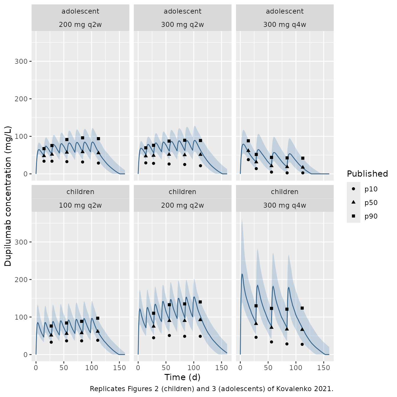
The simulated medians are compared with the digitised predicted medians below. The bins on dosing days sit at trough level, so the visits are treated as pre-dose samples: a bin within 1.5 days of a scheduled dose is evaluated just before that dose. For children the loading doses are assumed, so only the day-111 bin, where the loading dose has largely washed out, is gated; the earlier children bins are shown for information. All adolescent bins are gated because the adolescent regimens, loading doses included, are documented.
cmp_fig <- fig |>
  select(age, arm, time, t_eval, p50_pub = p50) |>
  left_join(pct |> select(age, arm, t_eval = time, p50_sim = p50), by = c("age", "arm", "t_eval")) |>
  mutate(
    pct_diff = 100 * (p50_sim / p50_pub - 1),
    gated = age == "adolescent" | time > 100
  )

cmp_fig |>
  mutate(across(c(p50_sim, pct_diff), ~ round(.x, 1))) |>
  rename(
    "Age group" = age, "Arm" = arm, "Time (d)" = time, "Evaluated at (d)" = t_eval,
    "Published median (mg/L)" = p50_pub, "Simulated median (mg/L)" = p50_sim,
    "Difference (%)" = pct_diff, "Gated" = gated
  ) |>
knitr::kable(caption = "Predicted medians: simulation vs digitised Figures 2 and 3.")| Age group | Arm | Time (d) | Evaluated at (d) | Published median (mg/L) | Simulated median (mg/L) | Difference (%) | Gated |
|---|---|---|---|---|---|---|---|
| children | 100 mg q2w | 27.4 | 27.99 | 51.3 | 49.1 | -4.2 | FALSE |
| children | 100 mg q2w | 55.0 | 55.99 | 55.7 | 54.6 | -2.0 | FALSE |
| children | 100 mg q2w | 82.1 | 82.10 | 57.5 | 61.9 | 7.7 | FALSE |
| children | 100 mg q2w | 111.0 | 111.00 | 61.4 | 61.2 | -0.4 | TRUE |
| children | 200 mg q2w | 27.8 | 27.99 | 75.0 | 80.6 | 7.5 | FALSE |
| children | 200 mg q2w | 56.1 | 55.99 | 90.1 | 92.4 | 2.6 | FALSE |
| children | 200 mg q2w | 83.6 | 83.99 | 90.2 | 97.5 | 8.1 | FALSE |
| children | 200 mg q2w | 111.7 | 111.70 | 92.3 | 103.1 | 11.7 | TRUE |
| children | 300 mg q4w | 28.3 | 27.99 | 82.0 | 84.0 | 2.5 | FALSE |
| children | 300 mg q4w | 56.1 | 55.99 | 71.8 | 75.0 | 4.5 | FALSE |
| children | 300 mg q4w | 83.8 | 83.99 | 67.3 | 71.4 | 6.1 | FALSE |
| children | 300 mg q4w | 111.3 | 111.30 | 66.2 | 71.1 | 7.4 | TRUE |
| adolescent | 200 mg q2w | 14.4 | 13.99 | 47.9 | 48.3 | 0.8 | TRUE |
| adolescent | 200 mg q2w | 28.7 | 27.99 | 51.8 | 52.9 | 2.1 | TRUE |
| adolescent | 200 mg q2w | 55.5 | 55.99 | 57.2 | 56.7 | -0.8 | TRUE |
| adolescent | 200 mg q2w | 83.8 | 83.99 | 58.5 | 58.3 | -0.3 | TRUE |
| adolescent | 200 mg q2w | 112.3 | 112.30 | 55.7 | 58.7 | 5.5 | TRUE |
| adolescent | 300 mg q2w | 13.7 | 13.99 | 47.4 | 51.6 | 8.9 | TRUE |
| adolescent | 300 mg q2w | 27.7 | 27.99 | 48.8 | 55.4 | 13.4 | TRUE |
| adolescent | 300 mg q2w | 55.6 | 55.99 | 51.6 | 60.7 | 17.5 | TRUE |
| adolescent | 300 mg q2w | 83.7 | 83.99 | 50.4 | 62.1 | 23.3 | TRUE |
| adolescent | 300 mg q2w | 112.1 | 112.10 | 51.3 | 62.9 | 22.6 | TRUE |
| adolescent | 300 mg q4w | 14.4 | 14.40 | 61.6 | 58.3 | -5.4 | TRUE |
| adolescent | 300 mg q4w | 28.7 | 27.99 | 31.4 | 31.7 | 0.9 | TRUE |
| adolescent | 300 mg q4w | 56.1 | 55.99 | 21.2 | 22.4 | 5.6 | TRUE |
| adolescent | 300 mg q4w | 84.2 | 83.99 | 18.6 | 18.2 | -2.0 | TRUE |
| adolescent | 300 mg q4w | 112.4 | 112.40 | 17.3 | 15.9 | -8.2 | TRUE |
gated <- cmp_fig |> filter(gated)
stopifnot(
  !anyNA(gated$p50_sim),
  nrow(gated) == 18L,
  # A mis-transcribed volume, rate constant or dose moves every median by tens
  # of percent; the virtual covariate distributions and the digitisation move
  # it by a few.
  abs(median(gated$pct_diff)) < 10,
  quantile(abs(gated$pct_diff), 0.9) < 30
)
Most bins agree within 10%. The adolescent 300 mg q2w arm (weight >= 60 kg) is over-predicted, increasingly over time, by roughly 10-25%. That arm is the heaviest group, where the virtual cohort is least certain: BMI is drawn independently of weight, so the heavy adolescents are not given the higher BMI (and hence faster linear elimination) they would have, and the upper tail of the trial’s weight distribution is not published.
PKNCA validation: steady-state trough
The Discussion states that the minimal model-predicted median steady-state trough concentration across the pediatric q2w groups is about 57 mg/L. The four q2w groups are simulated to steady state (26 doses) with the base models, which the Supplement describes as the models used for simulation, and the trough, peak and average concentration over the last dosing interval are computed with PKNCA.
ss_arms <- arms |> filter(tau == 14)
ss_last <- 14 * 25
ss_events <- bind_rows(lapply(seq_len(nrow(ss_arms)), function(i) {
  a <- ss_arms[i, ]
  wd <- wt_dist[[a$age]]
  subj <- tibble(
    id = (i - 1L) * n_per_arm + seq_len(n_per_arm),
    WT = draw_wt(n_per_arm, wd[1], wd[2], a$wt_lo, a$wt_hi)
  )
  doses <- tidyr::crossing(subj, time = seq(0, ss_last, by = 14)) |>
    mutate(amt = ifelse(time == 0, 2 * a$dose, a$dose), evid = 1L, cmt = "depot")
  obs <- tidyr::crossing(subj, time = c(0, ss_last + c(0, 0.25, 0.5, 1:14))) |>
    mutate(amt = 0, evid = 0L, cmt = "central")
  bind_rows(doses, obs) |>
    mutate(age = a$age, arm = a$arm, group = paste(a$age, a$arm)) |>
    arrange(id, time, desc(evid))
}))

ss_sim <- bind_rows(lapply(c("children", "adolescent"), function(ag) {
  mod <- readModelDb(models[[paste0(ag, "_base")]])
  as.data.frame(rxode2::rxSolve(mod, events = ss_events |> filter(age == ag),
                                keep = c("group"), returnType = "data.frame"))
}))
nca_conc <- ss_sim |>
  filter(!is.na(Cc)) |>
  select(id, time, Cc, group)
nca_conc <- bind_rows(
  nca_conc,
  nca_conc |> distinct(id, group) |> mutate(time = 0, Cc = 0)
) |>
  distinct(id, group, time, .keep_all = TRUE) |>
  arrange(id, group, time)

nca_dose <- ss_events |>
  filter(evid == 1) |>
  select(id, time, amt, group)

conc_obj <- PKNCA::PKNCAconc(nca_conc, Cc ~ time | group + id)
dose_obj <- PKNCA::PKNCAdose(nca_dose, amt ~ time | group + id)
intervals <- data.frame(
  start = ss_last, end = ss_last + 14,
  cmax = TRUE, cmin = TRUE, cav = TRUE
)
nca_res <- PKNCA::pk.nca(PKNCA::PKNCAdata(conc_obj, dose_obj, intervals = intervals))

ss_summary <- as.data.frame(nca_res) |>
  filter(PPTESTCD %in% c("cmin", "cmax", "cav")) |>
  group_by(group, PPTESTCD) |>
  summarise(median = median(PPORRES), .groups = "drop") |>
  pivot_wider(names_from = PPTESTCD, values_from = median)

ss_summary |>
  mutate(across(c(cmin, cmax, cav), ~ round(.x, 1))) |>
  rename(
    "Group" = group, "Median Ctrough,ss (mg/L)" = cmin,
    "Median Cmax,ss (mg/L)" = cmax, "Median Cavg,ss (mg/L)" = cav
  ) |>
knitr::kable(caption = "Simulated steady-state exposure in the pediatric q2w groups (base models).")| Group | Median Cavg,ss (mg/L) | Median Cmax,ss (mg/L) | Median Ctrough,ss (mg/L) |
|---|---|---|---|
| adolescent 200 mg q2w | 79.2 | 88.9 | 64.7 |
| adolescent 300 mg q2w | 67.8 | 78.3 | 53.2 |
| children 100 mg q2w | 86.1 | 104.6 | 65.9 |
| children 200 mg q2w | 123.8 | 152.1 | 96.4 |
sim_min <- data.frame(
  quantity = "Minimum median Ctrough,ss across pediatric q2w groups",
  cmin = min(ss_summary$cmin)
)
published_min <- data.frame(
  quantity = "Minimum median Ctrough,ss across pediatric q2w groups",
  cmin = 57
)
cmp <- nlmixr2lib::ncaComparisonTable(
  simulated = sim_min,
  reference = published_min,
  by = "quantity",
  units = c(cmin = "mg/L"),
  tolerance_pct = 20
)
knitr::kable(cmp, caption = "Simulated vs published (Discussion) minimum median steady-state trough. * differs by >20%.")| NCA parameter | quantity | Reference | Simulated | % diff |
|---|---|---|---|---|
| Cmin (mg/L) | Minimum median Ctrough,ss across pediatric q2w groups | 57 | 53.2 | -6.6% |
The lowest median steady-state trough is in the adolescent 300 mg q2w group, consistent with the adolescent q2w arms having the lowest troughs in Figure 3.
Covariate effects in the covariate models
The covariate models quote Vc and ke at the covariate central values. The table shows the multiplicative change in Vc or ke between the 10th and 90th percentiles of the virtual cohort’s covariates, which is independent of the central value chosen.
q <- function(x) quantile(x, c(0.1, 0.9))
ch <- events |> filter(age == "children") |> distinct(id, WT, ALB, SCORE_EASI)
ad <- events |> filter(age == "adolescent") |> distinct(id, WT, BMI, SCORE_EASI)
eff <- tribble(
  ~model, ~effect, ~ratio_p90_p10,
  "children", "WT on Vc", unname(diff(log(q(ch$WT))) * 0.849),
  "children", "ALB on Vc", unname(diff(log(q(ch$ALB))) * -0.525),
  "children", "EASI on ke", unname(diff(log(q(ch$SCORE_EASI))) * 0.169),
  "adolescent", "WT on Vc", unname(diff(log(q(ad$WT))) * 0.755),
  "adolescent", "BMI on ke", unname(diff(log(q(ad$BMI))) * 0.357),
  "adolescent", "EASI on ke", unname(diff(log(q(ad$SCORE_EASI))) * 0.356)
) |>
  mutate(ratio_p90_p10 = round(exp(ratio_p90_p10), 2))
eff |>
  rename("Age group" = model, "Effect" = effect, "Parameter ratio, 90th vs 10th percentile" = ratio_p90_p10) |>
knitr::kable()| Age group | Effect | Parameter ratio, 90th vs 10th percentile |
|---|---|---|
| children | WT on Vc | 1.90 |
| children | ALB on Vc | 0.90 |
| children | EASI on ke | 1.12 |
| adolescent | WT on Vc | 1.83 |
| adolescent | BMI on ke | 1.28 |
| adolescent | EASI on ke | 1.32 |
As the article concludes, body weight is the only covariate with a large effect (on Vc); the other effects change Vc or ke by about a third or less across the central 80% of the covariate range.
Assumptions and deviations
-
Covariate central values not printed. The article
states the weight central value (75 kg) but not those of albumin, BMI or
EASI (“median or another selected level of covariate”). The maintainers
used: albumin 44 g/L (a rounded standard, the same value used by
Kovalenko_2020_dupilumab_covariate); children EASI 37, the rounded baseline EASI mean of the dupilumab arms of LIBERTY AD PEDS (Siegfried 2023, Am J Clin Dermatol 24:787, Table 1: 37.1 and 37.4); adolescent EASI 36 and BMI 24.5 kg/m^2, the baseline means of the dupilumab arms of LIBERTY AD ADOL (Simpson 2020, JAMA Dermatol 156:44, Table 1). These are trial means, not the PK-analysis-set medians. A power-model central value does not change any covariate ratio; it changes only the covariate values at which the printed Vc and ke apply. -
Vm in the children base model. Table 1 labels the
children Vm “1.64 (fixed)”, but its footnote gives an SE “where it was
estimated rather than fixed” and the Methods state that Vm was estimated
in the base model and fixed in the covariate model. Vm is therefore an
estimated parameter in
Kovalenko_2021_dupilumab_children_baseandfixed()inKovalenko_2021_dupilumab_children_covariate. -
Transit chain. Figure 1 shows the dose passing
through three transit compartments spanned by MTT into an absorption
depot. The packaged models use three transfers at
ktr = 3 / MTT, so that MTT is the mean time spent in the chain, matching theNN = 3,KTR = NN / MTTconvention of the same group’s later deposited dupilumab control stream (Nguyen 2026,Nguyen_2026_dupilumab). With MTT = 0.105 d, the choice has no visible effect on concentrations. -
Residual error form. The supplement gives
proportional and additive standard deviations without stating how they
are combined; the models use nlmixr2’s default combined form, as in the
adult sibling models. Monolix’s
combined1form (standard deviations added,a + b * f) is the other possibility; it matters only in the adolescent models, where the additive term (2.4 mg/L) is not negligible. - Supplementary Table 1 inconsistency. Supplementary Table 1 swaps the patient and sample counts and the weight-banded doses between the two studies relative to the Methods text, which (together with the trial reports) was followed here.
- Virtual cohort. Covariate distributions are approximations (see Virtual cohort); the covariates are drawn independently of weight, and the children’s loading doses (twice the maintenance dose) are assumed.
- Not packaged. The clearance-parameterised sensitivity models (Tables 3 and 4) and the sensitivity analyses with median-weight centring, re-estimated Vm or F fixed to 1 are robustness checks, not primary models.
- No erratum or correction notice for this article was found as of 2026-09-29.