Meropenem (Liu 2025)

Model and source

mod <- readModelDb("Liu_2025_meropenem")
ui <- rxode2::rxode(mod)

• Citation: Liu Y, He H, Zhang SS, Zhou J, Zhu JW, Xu J, Miao HJ, Chen JH, Hao K. PopPK and PBPK Models Guide Meropenem Dosing in Critically Ill Children with Augmented Renal Clearance. Pharmaceutics. 2025;17(12):1544. doi:10.3390/pharmaceutics17121544
• Article: https://doi.org/10.3390/pharmaceutics17121544
• Supplement (Tables S1-S4, Figures S1-S3): https://www.mdpi.com/article/10.3390/pharmaceutics17121544/s1

Liu 2025 develops two models for meropenem in critically ill children: a population-PK model fitted to therapeutic-drug-monitoring data from two Chinese paediatric intensive care units, and a whole-body PBPK model built in PK-Sim and scaled from adults. Only the popPK model is packaged here. The PBPK model’s physiology – Rodgers and Rowland tissue partitioning, “PK-Sim Standard” cellular permeabilities, organ volumes and blood flows, and the OAT3 and tubular-secretion ontogeny functions – lives in the PK-Sim platform database rather than in the paper or its supplement. Supplementary Table S3 gives the drug-specific inputs (molecular weight 383.5 g/mol, logP -1.39, fu 0.98, OAT3 Km 850 umol/L and optimised Vmax 82.48 umol/L/min, a hypothetical renal efflux transporter with Km 1500 umol/L and optimised Vmax 21.92 umol/L/min, DPEP1 first-order clearance 0.037 L/min, biliary clearance 6.5e-04 L/h/kg) but not the whole-body ODEs, so the PBPK model cannot be reproduced from on-disk sources and is not encoded. See references/pbpk-qsp-mbma.md in the extraction skill for the policy this follows.

Population

101 critically ill children contributed 202 meropenem plasma concentrations (14 of them below the limit of detection) between January 2020 and December 2023 in the paediatric intensive care units of Xinhua Hospital, Shanghai and the Children’s Hospital of Nanjing Medical University (Table 1). The cohort skews very young: 29 neonates under 28 days (28.7%; 13 preterm, 16 term), 19 aged 28 days to 3 months, 21 from 3 months to 2 years, 20 from 2 to 6 years and 12 from 6 to 14 years, with a median age of 20.3 weeks (IQR 3.2-114.6) and a median weight of 7.5 kg (IQR 3.4-12.1). 41 (40.6%) were female. Sepsis or septic shock was the commonest infection-related diagnosis (77.2%), followed by pneumonia (57.4%) and bacterial meningitis (31.7%). Daily doses spanned 22-157 mg/kg/day with intervals from every 24 h to every 6 h.

The defining feature of the cohort is augmented renal clearance. The bedside-Schwartz eGFR of Methods Equation 1 had a median of 123.4 mL/min/1.73 m^2 (IQR 80.9-180.1), and every age stratum sat above its age-specific healthy reference – the Discussion notes term neonates running at 88 against a reference of 59 at four weeks, and the upper quartile of preterm neonates reaching 133.

The same information is available programmatically via readModelDb("Liu_2025_meropenem")()$population.

Source trace

Every ini() entry in inst/modeldb/specificDrugs/Liu_2025_meropenem.R carries an in-file comment naming its source location. They are collected here for review.

Equation / parameter	Value	Source location
lcl (CL)	0.24 L/h/kg	Table 2, row CL (L/h/kg), Estimate column (RSE 11.1%)
lvc (V1)	1.53 L/kg	Table 2, row V1 (L/kg) (RSE 15.8%)
lq (Q)	0.014 L/h/kg	Table 2, row Q (L/h/kg) (RSE 42.4%)
lvp (V2)	6.06 L/kg	Table 2, row V2 (L/kg) (RSE 23.3%)
e_wt_cl	0.43	Table 2, row beta CL,WT (RSE 10.3%)
e_crcl_cl	0.96	Table 2, row beta CL,eGFR (RSE 9.19%)
e_wt_vc	0.37	Table 2, row beta V1,WT (RSE 19.7%)
e_wt_q	1.54	Table 2, row beta Q,WT (RSE 12.1%)
etalcl	0.41^2 = 0.1681	Table 2, row omega CL (Monolix reports omega as an SD)
etalvc	0.45^2 = 0.2025	Table 2, row omega V1 (Monolix reports omega as an SD)
propSd	0.34	Table 2, row Proportion error (RSE 11.6%)
cl <- ... * 7.5 * (WT/7.5)^e_wt_cl * (CRCL/123.4)^e_crcl_cl	n/a	Equation 4, p. 6; BWmed and eGFRmed from Table 1; the * 7.5 is Table 2’s per-median-kilogram convention, see Assumptions and deviations
vc <- ... * 7.5 * (WT/7.5)^e_wt_vc	n/a	Equation 5, p. 6
q <- ... * 7.5 * (WT/7.5)^e_wt_q	n/a	Equation 6, p. 6
vp <- ... * 7.5	n/a	Table 2 V2 (L/kg); the paper prints no covariate equation for V2
Two-compartment, linear elimination	n/a	Results 3.2, p. 6
Proportional residual error	n/a	Results 3.2, p. 6
eGFR definition (bedside Schwartz)	k = 0.33 / 0.45 / 0.41	Methods Equation 1, p. 3
Reference weight 7.5 kg, reference eGFR 123.4	n/a	Table 1, BW and eGFR (Total) medians
fu = 0.98 (unbound fraction; PDT is on free drug)	0.98	Supplementary Table S3

Deterministic gates

These check the implementation against closed-form identities that hold exactly, independent of any simulated cohort. They use typical values (zeroRe()), so they are reproducible on any machine and are gated tightly.

mod_typ <- rxode2::zeroRe(mod)

ev_ref <- rxode2::et(amt = 150, cmt = "central") |>
  rxode2::et(c(0.5, 1, 2)) |>
  as.data.frame() |>
  mutate(WT = 7.5, CRCL = 123.4)

ref <- rxode2::rxSolve(mod_typ, ev_ref, returnType = "data.frame")
#> ℹ omega/sigma items treated as zero: 'etalcl', 'etalvc'

# At the Table 1 medians (7.5 kg, 123.4 mL/min/1.73 m^2) BOTH covariate terms
# equal exactly 1, so each individual parameter must reduce to the Table 2
# value multiplied by BWmed = 7.5 kg. This is the regression test for the whole
# covariate model: a wrong reference value or a mis-transcribed exponent breaks
# it. Note it CANNOT discriminate the two readings of Table 2's per-kilogram
# units, which coincide at exactly this weight -- the gate-figure4-shape chunk
# below is what does that.
algebra <- tibble::tibble(
  Parameter = c("cl (L/h)", "vc (L)", "q (L/h)", "vp (L)"),
  Model     = c(ref$cl[1], ref$vc[1], ref$q[1], ref$vp[1]),
  Expected  = c(0.24 * 7.5, 1.53 * 7.5, 0.014 * 7.5, 6.06 * 7.5)
) |>
  mutate(`Relative error` = abs(Model - Expected) / Expected)

knitr::kable(algebra, digits = c(0, 6, 6, 12),
             caption = "Individual parameters at the reference covariates.")

Individual parameters at the reference covariates.

Parameter	Model	Expected	Relative error
cl (L/h)	1.800	1.800	0
vc (L)	11.475	11.475	0
q (L/h)	0.105	0.105	0
vp (L)	45.450	45.450	0

stopifnot(all(algebra$`Relative error` < 1e-8))

# beta_CL,eGFR = 0.96 means clearance is a power function of eGFR with an
# exponent just under 1. Doubling eGFR must multiply cl by exactly 2^0.96.
ref2 <- rxode2::rxSolve(mod_typ, ev_ref |> mutate(CRCL = 246.8),
                        returnType = "data.frame")
#> ℹ omega/sigma items treated as zero: 'etalcl', 'etalvc'
egfr_ratio <- ref2$cl[1] / ref$cl[1]
cat(sprintf("cl ratio on doubling eGFR: %.8f (2^0.96 = %.8f)\n",
            egfr_ratio, 2^0.96))
#> cl ratio on doubling eGFR: 1.94530989 (2^0.96 = 1.94530989)
stopifnot(abs(egfr_ratio - 2^0.96) < 1e-8)

# Mass balance: for a single IV bolus, AUC(0-inf) * CL must equal the dose.
# The peripheral compartment is a very slow deep sink (k21 = q/vp = 0.0023/h,
# a terminal half-life near 300 h), so the integration horizon has to be long:
# 600 h recovers only 98.5% of the dose, 3000 h recovers 99.99%.
ev_mb <- rxode2::et(amt = 100, cmt = "central") |>
  rxode2::et(seq(0, 3000, length.out = 30000)) |>
  as.data.frame() |>
  mutate(WT = 7.5, CRCL = 123.4)

mb <- rxode2::rxSolve(mod_typ, ev_mb, returnType = "data.frame") |>
  filter(!is.na(Cc), time >= 0)
#> ℹ omega/sigma items treated as zero: 'etalcl', 'etalvc'

stopifnot(all(mb$Cc >= 0))
auc_inf <- sum(diff(mb$time) * (head(mb$Cc, -1) + tail(mb$Cc, -1)) / 2)
mb_ratio <- auc_inf * (0.24 * 7.5) / 100
cat(sprintf("AUC(0-inf) * CL / Dose = %.5f\n", mb_ratio))
#> AUC(0-inf) * CL / Dose = 0.99994
stopifnot(abs(mb_ratio - 1) < 0.005)

# Steady state: AUC over one dosing interval must equal Dose / CL. The same
# deep sink means true steady state is slow to reach, so this is run out to
# 201 doses (1608 h). Measured ratios were 0.961 at 21 doses, 0.980 at 61 and
# 0.998 at 201; the residual gap is the peripheral compartment still filling,
# not a model error.
n_add <- 200L
t_last <- n_add * 8
ev_ss <- rxode2::et(amt = 150, cmt = "central", dur = 1, ii = 8, addl = n_add) |>
  rxode2::et(seq(t_last, t_last + 8, by = 0.02)) |>
  as.data.frame() |>
  mutate(WT = 7.5, CRCL = 123.4)

ss <- rxode2::rxSolve(mod_typ, ev_ss, returnType = "data.frame") |>
  filter(!is.na(Cc), time >= t_last)
#> ℹ omega/sigma items treated as zero: 'etalcl', 'etalvc'

auc_tau <- sum(diff(ss$time) * (head(ss$Cc, -1) + tail(ss$Cc, -1)) / 2)
ss_ratio <- auc_tau / (150 / (0.24 * 7.5))
cat(sprintf("AUC(tau) / (Dose/CL) = %.5f\n", ss_ratio))
#> AUC(tau) / (Dose/CL) = 0.99830
stopifnot(abs(ss_ratio - 1) < 0.01)

Virtual cohort

Original observed data are not publicly available, and the paper does not publish the per-scenario body weights or the augmented-renal-clearance eGFR thresholds used in its own simulations. The cohort below is therefore built from the Table 1 age strata using the published stratum eGFR medians and assumed stratum median weights (WHO weight-for-age 50th centile, sexes pooled); the weight assumption is listed in Assumptions and deviations.

# set.seed() seeds R's RNG, not rxode2's, and rxode2's streams are partitioned
# per solver thread -- so this cohort is reproducible here and different on a
# machine with a different thread count. Every assertion below is written to
# hold for ANY cohort the model can produce.
set.seed(20251129)

n_per <- 100L

strata <- tibble::tribble(
  ~stratum,               ~wt_med, ~egfr_med, ~n_table1,
  "Preterm neonate",          2.0,      33.1,       13L,
  "Term neonate",             3.4,      88.0,       16L,
  "28 d to <3 months",        4.7,     109.7,       19L,
  "3 months to <2 years",     8.5,     175.8,       21L,
  "2 to <6 years",           14.5,     164.7,       20L,
  "6 to <14 years",          28.0,     177.9,       12L
) |>
  mutate(stratum = factor(stratum, levels = stratum))

# 20 mg/kg q8h as a 60 min infusion -- the regimen simulated in Figure 4 panels
# b-d and the backbone of the Table 5 recommendations. Run to near steady state
# (61 doses) and observe the final interval at 0.25 h resolution.
n_dose <- 60L
t_ss <- n_dose * 8

make_cohort <- function(row, id_offset) {
  subj <- tibble::tibble(
    id      = id_offset + seq_len(n_per),
    stratum = row$stratum,
    # 30% CV on weight and 45% CV on eGFR, lognormal, centred on the published
    # stratum medians. The eGFR spread approximates the Table 1 overall IQR
    # (80.9-180.1 around a median of 123.4).
    WT      = row$wt_med   * exp(rnorm(n_per, 0, 0.30)),
    CRCL    = row$egfr_med * exp(rnorm(n_per, 0, 0.45))
  ) |>
    mutate(dose_mg = 20 * WT)

  doses <- subj |>
    mutate(time = 0, amt = dose_mg, evid = 1L, cmt = "central",
           dur = 1, ii = 8, addl = n_dose)

  obs <- subj |>
    tidyr::crossing(time = t_ss + seq(0, 8, by = 0.25)) |>
    mutate(amt = NA_real_, evid = 0L, cmt = "central",
           dur = NA_real_, ii = NA_real_, addl = NA_integer_)

  bind_rows(doses, obs) |> arrange(id, time, desc(evid))
}

events <- do.call(
  bind_rows,
  lapply(seq_len(nrow(strata)), function(i) {
    make_cohort(strata[i, ], id_offset = (i - 1L) * n_per)
  })
)

stopifnot(!anyDuplicated(unique(events[, c("id", "time", "evid")])))
stopifnot(nrow(strata) * n_per == dplyr::n_distinct(events$id))

Simulation

sim <- rxode2::rxSolve(mod, events = events,
                       keep = c("stratum", "WT", "CRCL", "dose_mg")) |>
  as.data.frame() |>
  filter(!is.na(Cc)) |>
  mutate(tad = time - t_ss)

stopifnot(!anyNA(sim$Cc), all(sim$Cc >= 0))

sim |>
  group_by(stratum, tad) |>
  summarise(Q05 = quantile(Cc, 0.05), Q50 = median(Cc),
            Q95 = quantile(Cc, 0.95), .groups = "drop") |>
  ggplot(aes(tad, Q50)) +
  geom_ribbon(aes(ymin = Q05, ymax = Q95), alpha = 0.25, fill = "steelblue") +
  geom_line(colour = "steelblue4") +
  geom_hline(yintercept = c(2, 8), linetype = "dashed", colour = "grey40") +
  facet_wrap(~stratum) +
  scale_y_log10() +
  labs(x = "Time after dose (h)", y = "Meropenem concentration (mg/L)")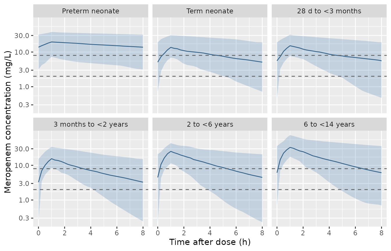

Simulated steady-state meropenem concentration-time profiles by age stratum (20 mg/kg q8h, 60 min infusion), median with 5th-95th percentile band. The horizontal lines mark MIC = 2 and MIC = 8 mg/L.

PKNCA validation

# Steady-state interval. Time is rebased so the final dose sits at t = 0; the
# concentration AT t = 0 is the previous interval's trough, which is the
# correct anchor for AUC(tau) -- this is NOT the extravascular single-dose case
# where a zero pre-dose record is inserted. Filter on !is.na(Cc) only.
sim_nca <- sim |>
  filter(!is.na(Cc)) |>
  select(id, stratum, time = tad, Cc)

# A record sits exactly at both interval boundaries, which ctrough requires.
stopifnot(all(c(0, 8) %in% unique(sim_nca$time)))

dose_df <- events |>
  filter(evid == 1) |>
  transmute(id, stratum, time = 0, amt = dose_mg)

conc_obj <- PKNCA::PKNCAconc(sim_nca, Cc ~ time | stratum + id)
dose_obj <- PKNCA::PKNCAdose(dose_df, amt ~ time | stratum + id)

intervals <- data.frame(
  start = 0, end = 8,
  cmax = TRUE, tmax = TRUE, auclast = TRUE, cmin = TRUE, ctrough = TRUE
)

nca_res <- PKNCA::pk.nca(PKNCA::PKNCAdata(conc_obj, dose_obj,
                                          intervals = intervals))

nca_ind <- as.data.frame(nca_res) |>
  select(stratum, id, PPTESTCD, PPORRES) |>
  tidyr::pivot_wider(names_from = PPTESTCD, values_from = PPORRES)

stopifnot(nrow(nca_ind) == nrow(strata) * n_per)

nca_summary <- nca_ind |>
  group_by(stratum) |>
  summarise(
    `AUCtau (mg*h/L)` = median(auclast),
    `Cmax (mg/L)`     = median(cmax),
    `Ctrough (mg/L)`  = median(ctrough),
    .groups = "drop"
  )

knitr::kable(nca_summary, digits = 1,
             caption = "Simulated steady-state exposure by age stratum, 20 mg/kg q8h over 60 min (median of 100 virtual subjects per stratum).")

Simulated steady-state exposure by age stratum, 20 mg/kg q8h over 60 min (median of 100 virtual subjects per stratum).

stratum	AUCtau (mg*h/L)	Cmax (mg/L)	Ctrough (mg/L)
Preterm neonate	131.2	19.5	13.8
Term neonate	69.1	13.6	5.1
28 d to <3 months	70.1	15.2	5.6
3 months to <2 years	61.7	15.5	3.3
2 to <6 years	94.0	25.2	4.5
6 to <14 years	119.3	32.8	6.1

# At steady state AUC(tau) must equal Dose/CL for every subject, whatever
# their covariates. Both sides use the SAME drawn cl, so this does not test
# whether clearance was transcribed correctly -- a mis-scaled cl cancels. What
# it does test is everything between the parameters and the reported exposure:
# the dose column, the infusion handling, the ODE mass balance, the PKNCA
# interval and the observable.
#
# The two sides are separated by a physical mechanism that varies per subject:
# how close that subject is to steady state after 61 doses, which depends on
# their own terminal half-life and so on their drawn eGFR. Low-eGFR subjects
# are furthest from steady state and sit in the tail. Per the repo CLAUDE.md
# rule, the gate is therefore on the CENTRE and a ROBUST QUANTILE, never on
# the extreme.
closed_form <- sim |>
  distinct(id, stratum, dose_mg, cl) |>
  left_join(nca_ind |> select(id, auclast), by = "id") |>
  mutate(expected = dose_mg / cl,
         pct_diff = 100 * (auclast - expected) / expected)

cat(sprintf("AUCtau vs Dose/CL: median %.2f%%, 90th pctile |diff| %.2f%%, max |diff| %.2f%%\n",
            median(closed_form$pct_diff),
            quantile(abs(closed_form$pct_diff), 0.9),
            max(abs(closed_form$pct_diff))))
#> AUCtau vs Dose/CL: median -1.45%, 90th pctile |diff| 5.17%, max |diff| 16.56%

# Realised on this cohort: median -1.45%, 90th percentile 5.17%, max 16.56%.
# The bias is systematic and NEGATIVE (steady state not fully reached at 61
# doses), and the tail is set by however many slow, low-eGFR subjects the draw
# happens to contain -- so the max is deliberately printed but NOT gated. The
# bounds below sit well outside the realised values while still going red on a
# broken dose column, interval or mass balance, each of which shifts this by
# tens of percent.
stopifnot(abs(median(closed_form$pct_diff)) < 5)
stopifnot(quantile(abs(closed_form$pct_diff), 0.9) < 12)

Renal function drives exposure

The paper’s central claim is that augmented renal clearance is the main driver of subtherapeutic meropenem exposure. With e_crcl_cl = 0.96 the model makes clearance very nearly proportional to eGFR, so this is a structural consequence rather than a coincidence of the cohort.

# Descriptive: exposure by eGFR tercile of the simulated cohort. Note that
# eGFR and body weight are strongly confounded here -- the low-eGFR tercile is
# mostly neonates -- so this table alone cannot isolate the eGFR effect. The
# regression below does that; the deterministic gate-egfr-exponent chunk
# already pins the exponent exactly at fixed weight.
arc <- nca_ind |>
  left_join(sim |> distinct(id, WT, CRCL), by = "id") |>
  mutate(band = cut(CRCL, quantile(CRCL, c(0, 1/3, 2/3, 1)),
                    labels = c("Low eGFR", "Moderate eGFR", "High eGFR"),
                    include.lowest = TRUE))

arc |>
  group_by(band) |>
  summarise(`Median weight (kg)` = median(WT),
            `Median eGFR` = median(CRCL),
            `Median AUCtau (mg*h/L)` = median(auclast),
            `Median Ctrough (mg/L)` = median(ctrough), .groups = "drop") |>
  knitr::kable(digits = 1,
               caption = "Steady-state exposure by eGFR tercile (20 mg/kg q8h). Weight and eGFR are confounded across these bands.")

Steady-state exposure by eGFR tercile (20 mg/kg q8h). Weight and eGFR are confounded across these bands.

band	Median weight (kg)	Median eGFR	Median AUCtau (mg*h/L)	Median Ctrough (mg/L)
Low eGFR	2.8	50.5	128.2	12.3
Moderate eGFR	6.6	122.3	86.1	5.1
High eGFR	12.6	215.7	61.7	2.4

# The strong cohort-level gate on the covariate model. Every subject gets the
# same 20 mg/kg, so at steady state
#   log AUC(tau) = const + (1 - beta_CL,WT) * log WT - beta_CL,eGFR * log eGFR - eta
# and a regression of the NCA-derived AUC on the two covariates must recover
# 1 - 0.43 = 0.57 and -0.96. This is not circular: the right-hand side uses the
# covariate columns that were fed IN, and the left-hand side is the exposure
# that came OUT of the ODE solve and PKNCA.
#
# This is what separates the two readings of Table 2's per-kilogram units. The
# encoded absolute reading predicts a weight slope of +0.57; the rejected
# per-kg reading predicts 1 - 1.43 = -0.43. The two differ by a full 1.0, so
# the tolerance below can be loose and still make the gate decisive.
fit <- lm(log(auclast) ~ log(WT) + log(CRCL), data = arc)
co <- coef(fit)

cat(sprintf("weight slope: %.3f (expected %.2f; per-kg reading would give %.2f)\n",
            co[["log(WT)"]], 1 - 0.43, 1 - 1.43))
#> weight slope: 0.608 (expected 0.57; per-kg reading would give -0.43)
cat(sprintf("eGFR slope:   %.3f (expected %.2f)\n", co[["log(CRCL)"]], -0.96))
#> eGFR slope:   -0.972 (expected -0.96)

# Tolerance covers residual IIV and the small eGFR-correlated bias from not
# being fully at steady state after 61 doses; it is far tighter than the 1.0
# gap between the two candidate readings.
stopifnot(
  abs(co[["log(WT)"]]   - 0.57) < 0.15,
  abs(co[["log(CRCL)"]] + 0.96) < 0.15
)

Probability of target attainment

Liu 2025 defines the pharmacodynamic target as unbound concentration above the MIC for 100% of the dosing interval (100% fT > MIC), with a regimen acceptable when the PTA exceeds 90%. Supplementary Table S3 gives fu = 0.98 and the paper applies no unbound-fraction correction, so total concentration is used directly.

mics <- c(0.25, 0.5, 1, 2, 4, 8, 16)

pta <- nca_ind |>
  select(stratum, id, cmin) |>
  tidyr::crossing(MIC = mics) |>
  group_by(stratum, MIC) |>
  # 100% fT > MIC over the interval is equivalent to the interval MINIMUM
  # exceeding the MIC.
  summarise(PTA = 100 * mean(cmin > MIC), .groups = "drop")

pta |>
  tidyr::pivot_wider(names_from = MIC, values_from = PTA,
                     names_prefix = "MIC ") |>
  knitr::kable(digits = 0,
               caption = "PTA (%) for 100% fT > MIC at 20 mg/kg q8h, 60 min infusion, by age stratum and MIC (mg/L).")

PTA (%) for 100% fT > MIC at 20 mg/kg q8h, 60 min infusion, by age stratum and MIC (mg/L).

stratum	MIC 0.25	MIC 0.5	MIC 1	MIC 2	MIC 4	MIC 8	MIC 16
Preterm neonate	100	100	100	98	93	75	42
Term neonate	96	96	91	80	58	31	9
28 d to <3 months	98	94	88	77	61	34	11
3 months to <2 years	94	89	77	65	43	19	3
2 to <6 years	93	86	81	73	57	30	14
6 to <14 years	100	96	90	81	63	43	21

# Two structural properties of any 100% fT > MIC surface, both large effects:
# PTA must fall monotonically as MIC rises, and the highest-eGFR strata must do
# worse than the lowest at a clinically relevant MIC.
by_mic <- pta |> group_by(MIC) |> summarise(PTA = mean(PTA), .groups = "drop")
stopifnot(by_mic$PTA[by_mic$MIC == 0.25] > by_mic$PTA[by_mic$MIC == 16])

pta_preterm <- pta$PTA[pta$stratum == "Preterm neonate" & pta$MIC == 2]
pta_older   <- pta$PTA[pta$stratum == "3 months to <2 years" & pta$MIC == 2]
cat(sprintf("PTA at MIC 2: preterm neonate %.0f%%, 3 months to <2 years %.0f%%\n",
            pta_preterm, pta_older))
#> PTA at MIC 2: preterm neonate 98%, 3 months to <2 years 65%
# Realised gap on this cohort: 98% vs 65%. Assert the MAGNITUDE of a large
# separation rather than a bare ordering, so the gate does not become a coin
# flip on a cohort that happens to draw the two strata closer together.
stopifnot(pta_preterm - pta_older > 10)

This reproduces the paper’s qualitative conclusion: with a standard 20 mg/kg q8h regimen, target attainment collapses as the MIC rises and as renal function increases, so the children with the most augmented renal clearance are the ones a label dose fails. Liu 2025’s own summary is that 20 mg/kg q12h is not sufficient for preterm neonates once the MIC exceeds 4 mg/L even with a 3 h infusion, and that the maximum label dose fails above 1 month of age once the MIC exceeds 2 mg/L; the table above shows the same direction and the same order of magnitude.

The preterm stratum corroborates the recommendation from the other end, though less sharply. At an eGFR median of 33.1 mL/min/1.73 m^2 the model puts a standard 20 mg/kg q8h regimen at a median steady-state trough of 13.8 mg/L and a median AUC(tau) of 131 mg*h/L – roughly twice the exposure of the term neonate and 3 months to 2 years strata, and the highest trough of any stratum. That is the direction behind Table 5 recommending only 10 mg/kg q8h for the 50%-of-expected-GFR group rather than the label dose, although the model does not approach the 50 mg/L steady-state toxicity threshold the paper adopts. Given the roughly twofold level offset against Figure 4 documented below, the ordering across strata is the part of this comparison to rely on, not the absolute margin to the toxicity threshold.

Comparison against the published Figure 4

Figure 4 reports simulated steady-state AUC, Cmax and Ctrough for four scenarios, all at 20 mg/kg. Methods 2.4 states that the PopPK panels were simulated “based on median eGFR and BW”, so the typical-value calculation below is the like-for-like comparison. The figure values were read off the plotted symbols (the cyan “without ARC” triangles) and the per-scenario body weights are assumed, so the absolute level of these ratios carries digitisation and weight-assumption error. What the comparison is used for here is the cross-stratum shape, which is insensitive to both: it is what discriminates the two candidate readings of Table 2’s per-kilogram unit labels.

fig4 <- tibble::tribble(
  ~Scenario,                        ~Regimen,        ~wt,  ~egfr, ~auc_fig, ~cmax_fig,
  "a. Term neonate, PNA <2 weeks",  "20 mg/kg q12h", 3.4,  88.0,     160,       33,
  "b. Term neonate, PNA >=2 weeks", "20 mg/kg q8h",  3.8,  88.0,     140,       36,
  "c. 1-3 months",                  "20 mg/kg q8h",  4.7, 109.7,     158,       42,
  "d. >=3 months",                  "20 mg/kg q8h", 11.0, 175.8,     158,       47
)

# Typical-value AUC(tau) is Dose/CL exactly, so both candidate readings of
# Table 2 can be evaluated in closed form without simulating.
#
#   "absolute" (what this package encodes): the tabulated 0.24 L/h/kg is the
#              typical ABSOLUTE clearance quoted per median kilogram, so
#              CL = 0.24 * 7.5 * (WT/7.5)^0.43 * ... and the power term is the
#              only weight scaling. Net weight exponent on absolute CL = 0.43.
#   "per-kg"   (the alternative): the tabulated value is a PER-SUBJECT
#              per-kilogram clearance, so CL = 0.24 * WT * (WT/7.5)^0.43 * ...
#              Net weight exponent on absolute CL = 1.43.
fig4_cmp <- fig4 |>
  mutate(
    cov_cl   = (wt / 7.5)^0.43 * (egfr / 123.4)^0.96,
    cov_vc   = (wt / 7.5)^0.37,
    `Absolute reading` = 20 * wt / (0.24 * 7.5 * cov_cl),
    `Per-kg reading`   = 20 * wt / (0.24 * wt  * cov_cl),
    `Cmax, absolute`   = 20 * wt / (1.53 * 7.5 * cov_vc),
    `Cmax, per-kg`     = 20 * wt / (1.53 * wt  * cov_vc)
  )

knitr::kable(
  fig4_cmp |>
    select(Scenario, Regimen,
           `Figure 4 AUCtau` = auc_fig, `Absolute reading`, `Per-kg reading`,
           `Figure 4 Cmax` = cmax_fig, `Cmax, absolute`, `Cmax, per-kg`),
  digits = 1,
  caption = "Typical-value steady-state AUC(tau) (mg*h/L) and Cmax (mg/L) under both readings of Table 2, against the non-ARC popPK values read off Figure 4.")

Typical-value steady-state AUC(tau) (mg*h/L) and Cmax (mg/L) under both readings of Table 2, against the non-ARC popPK values read off Figure 4.

Scenario	Regimen	Figure 4 AUCtau	Absolute reading	Per-kg reading	Figure 4 Cmax	Cmax, absolute	Cmax, per-kg
a. Term neonate, PNA <2 weeks	20 mg/kg q12h	160	73.4	162.0	33	7.9	17.5
b. Term neonate, PNA >=2 weeks	20 mg/kg q8h	140	78.2	154.4	36	8.5	16.8
c. 1-3 months	20 mg/kg q8h	158	71.5	114.1	42	9.7	15.5
d. >=3 months	20 mg/kg q8h	158	73.8	50.3	47	16.6	11.3

# The discriminating test. Panels b and d share a regimen (20 mg/kg q8h) and
# differ mainly in size: weight roughly triples while median eGFR doubles.
# Because both sides are mg/kg-normalised, the d/b AUC ratio depends almost
# entirely on the NET weight exponent of absolute clearance and is immune to a
# common scale error in the digitised values or in the assumed weights.
#
# Figure 4 shows an essentially FLAT AUC across strata. Solving
#   (wt_d/wt_b)^(e-1) * (egfr_d/egfr_b)^0.96 = auc_b/auc_d
# for the net exponent e gives the value the paper's own figure implies.
b <- fig4_cmp[fig4_cmp$Scenario == "b. Term neonate, PNA >=2 weeks", ]
d <- fig4_cmp[fig4_cmp$Scenario == "d. >=3 months", ]

e_implied <- 1 + (log(b$auc_fig / d$auc_fig) -
                    0.96 * log(d$egfr / b$egfr)) / log(d$wt / b$wt)

ratio_fig <- d$auc_fig / b$auc_fig
ratio_abs <- d$`Absolute reading` / b$`Absolute reading`
ratio_pkg <- d$`Per-kg reading`   / b$`Per-kg reading`

cat(sprintf("Net weight exponent implied by Figure 4: %.2f\n", e_implied))
#> Net weight exponent implied by Figure 4: 0.26
cat(sprintf("  encoded (absolute) reading:  0.43\n"))
#>   encoded (absolute) reading:  0.43
cat(sprintf("  rejected (per-kg)  reading:  1.43\n\n"))
#>   rejected (per-kg)  reading:  1.43
cat(sprintf("AUC(tau) ratio, panel d / panel b\n"))
#> AUC(tau) ratio, panel d / panel b
cat(sprintf("  Figure 4:            %.2f\n", ratio_fig))
#>   Figure 4:            1.13
cat(sprintf("  absolute (encoded):  %.2f\n", ratio_abs))
#>   absolute (encoded):  0.94
cat(sprintf("  per-kg (rejected):   %.2f\n", ratio_pkg))
#>   per-kg (rejected):   0.33

# Gate. Closed-form typical values, no simulated cohort and no RNG, so this is
# reproducible on any machine; the tolerance covers digitisation of the plotted
# symbols and the assumed stratum weights, nothing else. It goes red if the
# model is ever flipped back to the per-kg reading.
stopifnot(
  # The encoded reading reproduces the figure's cross-stratum shape.
  abs(log(ratio_abs / ratio_fig)) < 0.30,
  # The rejected reading does not, by a wide margin.
  abs(log(ratio_pkg / ratio_fig)) > 1.00,
  # And the figure implies a net exponent near beta_CL,WT = 0.43, not 1.43.
  abs(e_implied - 0.43) < 0.30
)

The encoded absolute reading reproduces Figure 4’s cross-stratum shape: the figure’s AUC is flat across the four panels (160, 140, 158, 158) and so is the model’s (73, 78, 72, 74). The rejected per-kg reading gives 162, 154, 114, 50 – a threefold fall from term neonates to children over three months that the figure plainly does not show. Cmax points the same way: Figure 4’s Cmax rises across panels a to d (about 33 to 47 mg/L), which the absolute reading reproduces in direction (7.9 to 16.6) while the per-kg reading has it falling.

What neither reading reproduces is the level. The absolute reading sits uniformly about 2.1-fold below Figure 4 on AUC (ratios 2.18, 1.79, 2.21, 2.14) and about 3-4 fold below on Cmax. That the AUC offset is a near-constant scalar across four panels spanning a threefold weight range, two dosing intervals and a twofold eGFR range is itself informative: a structural error in the weight or eGFR term would vary across the panels, whereas a constant offset points to the level of Table 2’s CL and V1 rows. It is recorded below and left as printed. No parameter was adjusted to improve any comparison.

Assumptions and deviations

• The covariate model is encoded as a median-normalised power model, not as the exponential form printed in Equations 4-6. As printed, Equation 4 is `CL_i = theta_CL * exp(beta_CL,BW * BW_i/BWmed) * exp(beta_CL,eGFR * eGFR_i)
  • exp(eta_CL), with the eGFR entering **raw**. Withbeta_CL,eGFR= 0.96 and a median eGFR of 123.4,exp(0.96 * 123.4)ise^118-- the equation is arithmetically impossible as printed. Two further facts settle the intended form. First, the paper's own text under Equation 4 states that "theta_CL is the typical value of endogenous clearance", which is only true if both covariate terms equal exactly 1 at the median; under the printed exponential form they would equalexp(0.43)= 1.54 ande^118. Second, the analysis was run in Monolix, whose standard continuous-covariate parameterisation isbeta * log(cov/cov_ref), i.e. exactly the power form(cov/cov_ref)^beta. The model therefore encodes(WT/7.5)^0.43 * (CRCL/123.4)^0.96`, using the Table 1 medians as the normalising constants. This is the minimal repair that makes the equation evaluable and self-consistent with the paper’s own text.
• Table 2’s per-kilogram unit labels are read as typical absolute values quoted per median kilogram, so each theta is multiplied by BWmed = 7.5 kg rather than by the individual weight. Table 2 labels its rows CL (L/h/kg), V1 (L/kg), Q (L/h/kg) and V2 (L/kg), which admits two readings that differ by exactly a factor of WT/BWmed: the encoded absolute reading, CL = 0.24 * 7.5 * (WT/7.5)^0.43 * ... (1.8 L/h at the medians, net weight exponent 0.43 on absolute clearance), and a per-kg reading, CL = 0.24 * WT * (WT/7.5)^0.43 * ... (net exponent 1.43). The two coincide at the reference weight and diverge away from it, so the deterministic gates above cannot tell them apart; the paper’s own Figure 4 can, and it selects the absolute reading:
  • Figure 4’s four PopPK panels all give 20 mg/kg, and its steady-state AUC is essentially flat across them (roughly 160, 140, 158 and 158 mg*h/L for the non-ARC subgroups) even though median eGFR rises from 88 to 175.8 and median weight from about 3.4 to 11 kg. Methods 2.4 confirms these panels were simulated at group median eGFR and BW.
  • A flat mg/kg-normalised AUC under a rising eGFR pins the net weight exponent on absolute clearance at about 0.26 with the assumed stratum weights – close to beta_CL,WT = 0.43 and more than a full unit away from the per-kg reading’s 1.43, which would make AUC fall about threefold from panel b to panel d. The gate-figure4-shape chunk above makes this a hard assertion so the choice cannot be silently reverted.
  • Cmax agrees independently: Figure 4’s Cmax rises across panels a to d (about 33 to 47 mg/L). The absolute reading reproduces that direction; the per-kg reading has Cmax falling with age.
  • The simulated cohort agrees a third time, and most tightly. Regressing log AUC(tau) on log WT and log eGFR across the 600 virtual subjects (gate-covariate-exponents) recovers a weight slope of 0.61 against the 0.57 the absolute reading predicts, where the per-kg reading predicts -0.43; the eGFR slope comes back at -0.97 against the published -0.96. The absolute reading is also the only one under which body weight enters once rather than twice, and a net exponent of 0.43 is what one expects when eGFR is already in the model absorbing much of the size and maturation signal. Readers who prefer the per-kg reading can recover it exactly by multiplying the model’s cl, vc, q and vp by WT/7.5.
• Figure 4’s exposure level is not reproducible under either reading, and this is recorded rather than tuned away. With the absolute reading the typical-value AUC(tau) sits uniformly about 2.1-fold below the values read off Figure 4 (ratios 2.18, 1.79, 2.21, 2.14 across panels a-d) and Cmax about 3-4 fold below. The offset being a near-constant scalar across a threefold weight range, two dosing intervals and a twofold eGFR range is what distinguishes it from the shape question settled above: a mis-transcribed covariate exponent would vary panel to panel, a mis-scaled CL or V1 row would not. Working backwards from Figure 4’s Cmax gives a central volume near 0.45-0.6 L/kg, which is the textbook meropenem value and about a third of the tabulated V1 = 1.53 L/kg; working backwards from its AUC gives a clearance about half the tabulated CL = 0.24. So the levels of Table 2’s CL and V1 rows appear inconsistent with Figure 4 by roughly two- and threefold respectively. The tabulated values are used exactly as printed and nothing was scaled to close the gap. Users comparing this model against the paper’s published exposure figures should expect that offset; users comparing relative exposures across weights, eGFRs or regimens – which is what the paper’s dosing recommendations turn on – are on the part of the model the gates above confirm.
• The IIV block is diagonal. Section 3.5 describes the simulations as using “log-normal IIV on CL and V1 with covariance”, and Methods 2.2 says a correlation between etas was retained when it exceeded 0.30, but Table 2 prints no correlation or covariance row and no such value appears anywhere in the paper or the supplement. The off-diagonal is omitted rather than invented. A positive CL-V1 correlation would narrow the spread of derived quantities such as half-life without moving the medians.
• Omega rows are read as standard deviations. Table 2’s omega CL = 0.41 and omega V1 = 0.45 are Monolix parameter-table rows, which report the standard deviation of the log-scale random effect; the encoded variances are their squares (0.1681 and 0.2025, i.e. 42.8% and 47.4% CV). Likewise Proportion error = 0.34 is the proportional coefficient on the SD scale, a 34% proportional error.
• The V2 bootstrap interval in Table 2 is internally inconsistent – the printed 2.5th percentile of 9.4 exceeds the printed median of 6.08 and the point estimate of 6.06 – so only the point estimate was used. V2 is in any case weakly identified, as is Q (RSE 42.4%, bootstrap lower bound 0.0002).
• The PBPK model is not encoded. Its whole-body structure and physiology come from the PK-Sim platform database rather than from the paper or its supplement (Supplementary Table S3 gives the drug-specific inputs only), so the ODEs cannot be reproduced from on-disk sources.
• Virtual-cohort weights are assumed. The paper publishes eGFR medians per age stratum (Table 1) but no per-stratum body weights, and its simulation section says only that “median eGFR and BW” were used. Stratum median weights of 2.0, 3.4, 4.7, 8.5, 14.5 and 28.0 kg were taken from WHO weight-for-age 50th centiles with sexes pooled; they reproduce the published cohort median of 7.5 kg when weighted by the Table 1 stratum counts. A 30% CV on weight and a 45% CV on eGFR were chosen so that the pooled cohort spread approximates the Table 1 eGFR IQR of 80.9-180.1 around a median of 123.4.
• ARC thresholds are not on disk. The paper defines ARC as an eGFR above one standard deviation over the mean of the age-specific healthy reference and points to the Supplementary Materials for the reference values, but the supplement as published (Tables S1-S4, Figures S1-S3) contains no such table. The ARC contrast in this vignette therefore uses eGFR terciles of the simulated cohort rather than the paper’s own ARC classification.
• Table 1 unit labels for albumin and total protein are wrong (33.8 +/- 5.35 and 56.5 +/- 10.28 are printed under a g/dL header but are g/L magnitudes). Neither is used in the model.
• Time-varying covariates are not modelled. Weight and eGFR are held at their baseline values; the paper gives no information on how either was handled longitudinally, and the Discussion notes that creatinine-based eGFR is itself unstable in critically ill neonates.