Sunitinib and SU012662 PK and safety PK-PD in children (Wang 2020)

Model and source

• Citation: Wang E, DuBois SG, Wetmore C, Khosravan R. Population pharmacokinetics-pharmacodynamics of sunitinib in pediatric patients with solid tumors. Cancer Chemother Pharmacol. 2020;86(2):181-192. doi:10.1007/s00280-020-04106-z.
• Article: https://doi.org/10.1007/s00280-020-04106-z
• PD model structures: Khosravan 2016, Figure 5, https://doi.org/10.1007/s40262-016-0404-5

Wang 2020 pooled two Children’s Oncology Group trials of oral sunitinib in children and young adults with refractory solid tumours. It reports three kinds of model, and nlmixr2lib packages them as the authors built them, in ten files:

Model file	What it describes	Wang 2020 source
Wang_2020_sunitinib	Sunitinib (parent) two-compartment PK	Table 3, Results
Wang_2020_sunitinib_su12662	SU012662 (active metabolite) two-compartment PK, fitted separately	Table 3, Results
Wang_2020_sunitinib_anc	Absolute neutrophil count, transit/feedback model with Emax	Table 4
Wang_2020_sunitinib_plt	Platelet count, transit/feedback model with Emax	Table 4
Wang_2020_sunitinib_wbc	White blood cell count, transit/feedback model with Emax	Table 4
Wang_2020_sunitinib_lymphocytes	Lymphocyte count, transit/feedback model with Emax fixed to 1	Table 4
Wang_2020_sunitinib_hb	Hemoglobin, transit/feedback model with a linear drug effect	Table 4
Wang_2020_sunitinib_alt	ALT, indirect response with a linear drug effect on kout	Table 4
Wang_2020_sunitinib_ast	AST, indirect response with a linear drug effect on kout	Table 4
Wang_2020_sunitinib_dbp	Diastolic blood pressure, indirect response with a linear drug effect on kin	Table 4

The PK-PD models were fitted sequentially on the final sunitinib PK model’s predictions, so each PD file carries the sunitinib PK layer with its parameters wrapped in fixed(). The logistic-regression analyses of categorical adverse events (Wang 2020 Figure 2) report no coefficients and are not packaged.

Population

Fifty-nine patients aged 2-21 years (28 male, 31 female; 3 Asian, 53 non-Asian, 3 unknown) from studies ADVL0612 (n = 35) and ACNS1021 (n = 24) contributed data (Wang 2020 Table 2). Median body weight was 50.4 kg (16.2-100 kg) and median body surface area (BSA) 1.47 m^2 (0.66-2.14 m^2). Tumours were predominantly high-grade glioma, ependymoma, brain stem glioma or sarcoma. Patients received sunitinib 15 or 20 mg/m^2 once daily on schedule 4/2 (4 weeks on treatment, 2 weeks off). The analysis used 365 sunitinib and 340 SU012662 plasma concentrations.

The same information is available programmatically, e.g. readModelDb("Wang_2020_sunitinib")()$population.

Source trace

Every ini() value carries an in-file comment naming its table and row. The table below is generated from the packaged models: PK parameters come from Wang 2020 Table 3 and PD parameters from the named endpoint block of Table 4. Between-subject variability is printed as CV% in both tables and converted with omega^2 = log(1 + CV^2).

model_names <- c(
  "Wang_2020_sunitinib", "Wang_2020_sunitinib_su12662",
  paste0("Wang_2020_sunitinib_", c("anc", "plt", "wbc", "lymphocytes", "hb", "alt", "ast", "dbp"))
)
pk_names <- c("lka", "ltlag", "lcl", "lvc", "lvp", "lq", "e_bsa_cl", "e_bsa_vc", "etalcl", "etalvc", "etalka")
trace_one <- function(nm) {
  ui <- rxode2::rxode(readModelDb(nm))
  ini <- ui$iniDf
  ini <- ini[is.na(ini$neta2) | ini$neta1 == ini$neta2, ]
  is_pd_file <- !nm %in% model_names[1:2]
  src <- if (is_pd_file) {
    ifelse(ini$name %in% pk_names, "Table 3 (sunitinib PK layer)", "Table 4")
  } else {
    rep("Table 3", nrow(ini))
  }
  data.frame(
    Model = sub("Wang_2020_sunitinib_?", "", nm),
    Parameter = ini$name,
    Estimate = vapply(
      signif(ifelse(grepl("^l", ini$name) & is.na(ini$neta1), exp(ini$est), ini$est), 4),
      function(v) format(v, scientific = FALSE, drop0trailing = TRUE), character(1)
    ),
    Scale = ifelse(!is.na(ini$neta1), "omega^2", ifelse(grepl("^l", ini$name), "exp(value)", "value")),
    Fixed = ini$fix,
    Source = src
  )
}
trace <- dplyr::bind_rows(lapply(model_names, trace_one))
#> ℹ parameter labels from comments will be replaced by 'label()'
#> ℹ parameter labels from comments will be replaced by 'label()'
#> ℹ parameter labels from comments will be replaced by 'label()'
#> ℹ parameter labels from comments will be replaced by 'label()'
#> ℹ parameter labels from comments will be replaced by 'label()'
#> ℹ parameter labels from comments will be replaced by 'label()'
#> ℹ parameter labels from comments will be replaced by 'label()'
#> ℹ parameter labels from comments will be replaced by 'label()'
#> ℹ parameter labels from comments will be replaced by 'label()'
#> ℹ parameter labels from comments will be replaced by 'label()'
trace$Model[trace$Model == ""] <- "sunitinib PK"
stopifnot(
  all(trace$Source[trace$Model %in% c("sunitinib PK", "su12662")] == "Table 3"),
  all(trace$Source[trace$Parameter %in% c("lrbase", "propSd") & !trace$Model %in% c("sunitinib PK", "su12662")] == "Table 4")
)
knitr::kable(trace)

Model	Parameter	Estimate	Scale	Fixed	Source
sunitinib PK	lka	0.38	exp(value)	FALSE	Table 3
sunitinib PK	ltlag	0.64	exp(value)	FALSE	Table 3
sunitinib PK	lcl	24.1	exp(value)	FALSE	Table 3
sunitinib PK	lvc	1070	exp(value)	FALSE	Table 3
sunitinib PK	lvp	63.8	exp(value)	FALSE	Table 3
sunitinib PK	lq	0.28	exp(value)	FALSE	Table 3
sunitinib PK	e_bsa_cl	0.557	value	FALSE	Table 3
sunitinib PK	e_bsa_vc	1.47	value	FALSE	Table 3
sunitinib PK	propSd	0.319	value	FALSE	Table 3
sunitinib PK	etalcl	0.1106	omega^2	FALSE	Table 3
sunitinib PK	etalvc	0.05646	omega^2	FALSE	Table 3
sunitinib PK	etalka	0.5705	omega^2	FALSE	Table 3
su12662	lfdepot	0.21	exp(value)	TRUE	Table 3
su12662	lka	0.28	exp(value)	FALSE	Table 3
su12662	ltlag	0.46	exp(value)	FALSE	Table 3
su12662	lcl_su12662	10.9	exp(value)	FALSE	Table 3
su12662	lvc_su12662	1030	exp(value)	FALSE	Table 3
su12662	lvp_su12662	122	exp(value)	FALSE	Table 3
su12662	lq_su12662	17.8	exp(value)	FALSE	Table 3
su12662	e_bsa_cl_su12662	0.843	value	FALSE	Table 3
su12662	e_bsa_vc_su12662	1.72	value	FALSE	Table 3
su12662	propSd_su12662	0.231	value	FALSE	Table 3
su12662	etalcl_su12662	0.2081	omega^2	FALSE	Table 3
su12662	etalvc_su12662	0.2223	omega^2	FALSE	Table 3
su12662	etalka	0.4215	omega^2	FALSE	Table 3
anc	lka	0.38	exp(value)	TRUE	Table 3 (sunitinib PK layer)
anc	ltlag	0.64	exp(value)	TRUE	Table 3 (sunitinib PK layer)
anc	lcl	24.1	exp(value)	TRUE	Table 3 (sunitinib PK layer)
anc	lvc	1070	exp(value)	TRUE	Table 3 (sunitinib PK layer)
anc	lvp	63.8	exp(value)	TRUE	Table 3 (sunitinib PK layer)
anc	lq	0.28	exp(value)	TRUE	Table 3 (sunitinib PK layer)
anc	e_bsa_cl	0.557	value	TRUE	Table 3 (sunitinib PK layer)
anc	e_bsa_vc	1.47	value	TRUE	Table 3 (sunitinib PK layer)
anc	lrbase	3.7	exp(value)	FALSE	Table 4
anc	lmtt	207	exp(value)	FALSE	Table 4
anc	lemax	0.16	exp(value)	FALSE	Table 4
anc	lec50	1.8	exp(value)	FALSE	Table 4
anc	lhill	1	exp(value)	TRUE	Table 4
anc	lgamma	0.27	exp(value)	FALSE	Table 4
anc	propSd	0.388	value	FALSE	Table 4
anc	etalcl	0.1106	omega^2	TRUE	Table 3 (sunitinib PK layer)
anc	etalvc	0.05646	omega^2	TRUE	Table 3 (sunitinib PK layer)
anc	etalka	0.5705	omega^2	TRUE	Table 3 (sunitinib PK layer)
anc	etalrbase	0.2296	omega^2	FALSE	Table 4
anc	etalec50	1.018	omega^2	FALSE	Table 4
plt	lka	0.38	exp(value)	TRUE	Table 3 (sunitinib PK layer)
plt	ltlag	0.64	exp(value)	TRUE	Table 3 (sunitinib PK layer)
plt	lcl	24.1	exp(value)	TRUE	Table 3 (sunitinib PK layer)
plt	lvc	1070	exp(value)	TRUE	Table 3 (sunitinib PK layer)
plt	lvp	63.8	exp(value)	TRUE	Table 3 (sunitinib PK layer)
plt	lq	0.28	exp(value)	TRUE	Table 3 (sunitinib PK layer)
plt	e_bsa_cl	0.557	value	TRUE	Table 3 (sunitinib PK layer)
plt	e_bsa_vc	1.47	value	TRUE	Table 3 (sunitinib PK layer)
plt	lrbase	242	exp(value)	FALSE	Table 4
plt	lmtt	173	exp(value)	FALSE	Table 4
plt	lemax	0.14	exp(value)	FALSE	Table 4
plt	lec50	64.9	exp(value)	FALSE	Table 4
plt	lhill	1	exp(value)	TRUE	Table 4
plt	lgamma	0.19	exp(value)	FALSE	Table 4
plt	propSd	0.167	value	FALSE	Table 4
plt	etalcl	0.1106	omega^2	TRUE	Table 3 (sunitinib PK layer)
plt	etalvc	0.05646	omega^2	TRUE	Table 3 (sunitinib PK layer)
plt	etalka	0.5705	omega^2	TRUE	Table 3 (sunitinib PK layer)
plt	etalrbase	0.1106	omega^2	FALSE	Table 4
plt	etalec50	1.332	omega^2	FALSE	Table 4
wbc	lka	0.38	exp(value)	TRUE	Table 3 (sunitinib PK layer)
wbc	ltlag	0.64	exp(value)	TRUE	Table 3 (sunitinib PK layer)
wbc	lcl	24.1	exp(value)	TRUE	Table 3 (sunitinib PK layer)
wbc	lvc	1070	exp(value)	TRUE	Table 3 (sunitinib PK layer)
wbc	lvp	63.8	exp(value)	TRUE	Table 3 (sunitinib PK layer)
wbc	lq	0.28	exp(value)	TRUE	Table 3 (sunitinib PK layer)
wbc	e_bsa_cl	0.557	value	TRUE	Table 3 (sunitinib PK layer)
wbc	e_bsa_vc	1.47	value	TRUE	Table 3 (sunitinib PK layer)
wbc	lrbase	6.1	exp(value)	FALSE	Table 4
wbc	lmtt	230	exp(value)	FALSE	Table 4
wbc	lemax	0.1	exp(value)	FALSE	Table 4
wbc	lec50	7.1	exp(value)	FALSE	Table 4
wbc	lhill	1	exp(value)	TRUE	Table 4
wbc	lgamma	0.28	exp(value)	FALSE	Table 4
wbc	propSd	0.26	value	FALSE	Table 4
wbc	etalcl	0.1106	omega^2	TRUE	Table 3 (sunitinib PK layer)
wbc	etalvc	0.05646	omega^2	TRUE	Table 3 (sunitinib PK layer)
wbc	etalka	0.5705	omega^2	TRUE	Table 3 (sunitinib PK layer)
wbc	etalrbase	0.1682	omega^2	FALSE	Table 4
wbc	etalec50	1.911	omega^2	FALSE	Table 4
lymphocytes	lka	0.38	exp(value)	TRUE	Table 3 (sunitinib PK layer)
lymphocytes	ltlag	0.64	exp(value)	TRUE	Table 3 (sunitinib PK layer)
lymphocytes	lcl	24.1	exp(value)	TRUE	Table 3 (sunitinib PK layer)
lymphocytes	lvc	1070	exp(value)	TRUE	Table 3 (sunitinib PK layer)
lymphocytes	lvp	63.8	exp(value)	TRUE	Table 3 (sunitinib PK layer)
lymphocytes	lq	0.28	exp(value)	TRUE	Table 3 (sunitinib PK layer)
lymphocytes	e_bsa_cl	0.557	value	TRUE	Table 3 (sunitinib PK layer)
lymphocytes	e_bsa_vc	1.47	value	TRUE	Table 3 (sunitinib PK layer)
lymphocytes	lrbase	1.5	exp(value)	FALSE	Table 4
lymphocytes	lmtt	1990	exp(value)	FALSE	Table 4
lymphocytes	lemax	1	exp(value)	TRUE	Table 4
lymphocytes	lec50	165	exp(value)	FALSE	Table 4
lymphocytes	lhill	1	exp(value)	TRUE	Table 4
lymphocytes	lgamma	1	exp(value)	TRUE	Table 4
lymphocytes	propSd	0.243	value	FALSE	Table 4
lymphocytes	etalcl	0.1106	omega^2	TRUE	Table 3 (sunitinib PK layer)
lymphocytes	etalvc	0.05646	omega^2	TRUE	Table 3 (sunitinib PK layer)
lymphocytes	etalka	0.5705	omega^2	TRUE	Table 3 (sunitinib PK layer)
lymphocytes	etalrbase	0.2176	omega^2	FALSE	Table 4
lymphocytes	etalec50	2.852	omega^2	FALSE	Table 4
hb	lka	0.38	exp(value)	TRUE	Table 3 (sunitinib PK layer)
hb	ltlag	0.64	exp(value)	TRUE	Table 3 (sunitinib PK layer)
hb	lcl	24.1	exp(value)	TRUE	Table 3 (sunitinib PK layer)
hb	lvc	1070	exp(value)	TRUE	Table 3 (sunitinib PK layer)
hb	lvp	63.8	exp(value)	TRUE	Table 3 (sunitinib PK layer)
hb	lq	0.28	exp(value)	TRUE	Table 3 (sunitinib PK layer)
hb	e_bsa_cl	0.557	value	TRUE	Table 3 (sunitinib PK layer)
hb	e_bsa_vc	1.47	value	TRUE	Table 3 (sunitinib PK layer)
hb	lrbase	13	exp(value)	FALSE	Table 4
hb	lmtt	1370	exp(value)	FALSE	Table 4
hb	lslope	0.000317	exp(value)	FALSE	Table 4
hb	lgamma	1	exp(value)	TRUE	Table 4
hb	propSd	0.058	value	FALSE	Table 4
hb	etalcl	0.1106	omega^2	TRUE	Table 3 (sunitinib PK layer)
hb	etalvc	0.05646	omega^2	TRUE	Table 3 (sunitinib PK layer)
hb	etalka	0.5705	omega^2	TRUE	Table 3 (sunitinib PK layer)
hb	etalrbase	0.01453	omega^2	FALSE	Table 4
hb	etalslope	2.062	omega^2	FALSE	Table 4
alt	lka	0.38	exp(value)	TRUE	Table 3 (sunitinib PK layer)
alt	ltlag	0.64	exp(value)	TRUE	Table 3 (sunitinib PK layer)
alt	lcl	24.1	exp(value)	TRUE	Table 3 (sunitinib PK layer)
alt	lvc	1070	exp(value)	TRUE	Table 3 (sunitinib PK layer)
alt	lvp	63.8	exp(value)	TRUE	Table 3 (sunitinib PK layer)
alt	lq	0.28	exp(value)	TRUE	Table 3 (sunitinib PK layer)
alt	e_bsa_cl	0.557	value	TRUE	Table 3 (sunitinib PK layer)
alt	e_bsa_vc	1.47	value	TRUE	Table 3 (sunitinib PK layer)
alt	lrbase	26.5	exp(value)	FALSE	Table 4
alt	lkout	0.00559	exp(value)	FALSE	Table 4
alt	lslope	0.00443	exp(value)	FALSE	Table 4
alt	propSd	0.339	value	FALSE	Table 4
alt	etalcl	0.1106	omega^2	TRUE	Table 3 (sunitinib PK layer)
alt	etalvc	0.05646	omega^2	TRUE	Table 3 (sunitinib PK layer)
alt	etalka	0.5705	omega^2	TRUE	Table 3 (sunitinib PK layer)
alt	etalrbase	0.1822	omega^2	FALSE	Table 4
alt	etalkout	0.4054	omega^2	FALSE	Table 4
alt	etalslope	0.6721	omega^2	FALSE	Table 4
ast	lka	0.38	exp(value)	TRUE	Table 3 (sunitinib PK layer)
ast	ltlag	0.64	exp(value)	TRUE	Table 3 (sunitinib PK layer)
ast	lcl	24.1	exp(value)	TRUE	Table 3 (sunitinib PK layer)
ast	lvc	1070	exp(value)	TRUE	Table 3 (sunitinib PK layer)
ast	lvp	63.8	exp(value)	TRUE	Table 3 (sunitinib PK layer)
ast	lq	0.28	exp(value)	TRUE	Table 3 (sunitinib PK layer)
ast	e_bsa_cl	0.557	value	TRUE	Table 3 (sunitinib PK layer)
ast	e_bsa_vc	1.47	value	TRUE	Table 3 (sunitinib PK layer)
ast	lrbase	26.2	exp(value)	FALSE	Table 4
ast	lkout	1.7	exp(value)	FALSE	Table 4
ast	lslope	0.00492	exp(value)	FALSE	Table 4
ast	propSd	0.312	value	FALSE	Table 4
ast	etalcl	0.1106	omega^2	TRUE	Table 3 (sunitinib PK layer)
ast	etalvc	0.05646	omega^2	TRUE	Table 3 (sunitinib PK layer)
ast	etalka	0.5705	omega^2	TRUE	Table 3 (sunitinib PK layer)
ast	etalrbase	0.08344	omega^2	FALSE	Table 4
ast	etalkout	2.992	omega^2	FALSE	Table 4
ast	etalslope	0.0004409	omega^2	FALSE	Table 4
dbp	lka	0.38	exp(value)	TRUE	Table 3 (sunitinib PK layer)
dbp	ltlag	0.64	exp(value)	TRUE	Table 3 (sunitinib PK layer)
dbp	lcl	24.1	exp(value)	TRUE	Table 3 (sunitinib PK layer)
dbp	lvc	1070	exp(value)	TRUE	Table 3 (sunitinib PK layer)
dbp	lvp	63.8	exp(value)	TRUE	Table 3 (sunitinib PK layer)
dbp	lq	0.28	exp(value)	TRUE	Table 3 (sunitinib PK layer)
dbp	e_bsa_cl	0.557	value	TRUE	Table 3 (sunitinib PK layer)
dbp	e_bsa_vc	1.47	value	TRUE	Table 3 (sunitinib PK layer)
dbp	lrbase	65.9	exp(value)	FALSE	Table 4
dbp	lkout	0.017	exp(value)	FALSE	Table 4
dbp	lslope	0.00225	exp(value)	FALSE	Table 4
dbp	propSd	0.094	value	FALSE	Table 4
dbp	etalcl	0.1106	omega^2	TRUE	Table 3 (sunitinib PK layer)
dbp	etalvc	0.05646	omega^2	TRUE	Table 3 (sunitinib PK layer)
dbp	etalka	0.5705	omega^2	TRUE	Table 3 (sunitinib PK layer)
dbp	etalrbase	0.009174	omega^2	FALSE	Table 4
dbp	etalkout	0.8624	omega^2	FALSE	Table 4
dbp	etalslope	0.2272	omega^2	FALSE	Table 4

Model equations and their sources:

Equation	Source
Two-compartment disposition, first-order absorption with lag time (both analytes)	Wang 2020 Methods and Results; Table 3
CL/F = 24.1 * (1 + 0.557 * (BSA - 1.47)), Vc/F = 1070 * (BSA/1.47)^1.47 (sunitinib)	Wang 2020 Results
CL/F = 10.9 * (BSA/1.47)^0.843, Vc/F = 1030 * (BSA/1.47)^1.72 (SU012662)	Wang 2020 Results
21% of the sunitinib dose enters the SU012662 model	Wang 2020 Results (assumed conversion)
Proliferating pool, three transit compartments, circulating pool, Kprol = Ktr = Kcirc, feedback (BASE/circ)^POW	Khosravan 2016 Figure 5A (cited by Wang 2020 as the model source)
Ktr = 4 / MTT	Friberg 2002 convention (see Assumptions)
Edrug = Emax * C^GAM / (EC50^GAM + C^GAM) inhibiting Kprol	Wang 2020 Results; Table 4 (GAM fixed to 1)
Hemoglobin: Edrug = kPD * C inhibiting Kprol	Wang 2020 Results (see Assumptions)
ALT, AST: dR/dt = kin - kout * (1 - kPD * C) * R	Wang 2020 Results; Khosravan 2016 Figure 5B (see Assumptions)
DBP: dR/dt = kin * (1 + kPD * C) - kout * R	Wang 2020 Results; Khosravan 2016 Figure 5B (see Assumptions)
kin = BASE * kout, R(0) = BASE	steady-state baseline of an indirect-response model

Virtual cohort

Doses in the trials were BSA-based, so the virtual cohort draws a BSA for each subject from a log-normal distribution centred on the cohort median (1.47 m^2), redrawing any value outside the observed range 0.66-2.14 m^2. Two arms of 100 subjects receive 15 or 20 mg/m^2 once daily for the 28 days of a schedule-4/2 cycle.

set.seed(2020)
rxode2::rxSetSeed(2020)
n_per_arm <- 100

draw_bsa <- function(n) {
  out <- numeric(0)
  while (length(out) < n) {
    x <- exp(rnorm(n, log(1.47), 0.3))
    out <- c(out, x[x >= 0.66 & x <= 2.14])
  }
  out[seq_len(n)]
}

cohort <- data.frame(
  id = seq_len(2 * n_per_arm),
  dose_m2 = rep(c(15, 20), each = n_per_arm),
  BSA = draw_bsa(2 * n_per_arm)
)
cohort$dose_mg <- cohort$dose_m2 * cohort$BSA
cohort$treatment <- paste0(cohort$dose_m2, " mg/m^2")

summary(cohort$BSA)
#>    Min. 1st Qu.  Median    Mean 3rd Qu.    Max. 
#>  0.7398  1.1606  1.4281  1.4313  1.6910  2.1358

# Once-daily doses on days 1-28 plus observations on the named ODE state.
make_events <- function(cohort, obs_times, obs_cmt, n_doses = 28) {
  doses <- merge(cohort, data.frame(time = 24 * (seq_len(n_doses) - 1)))
  doses$amt <- doses$dose_mg
  doses$evid <- 1L
  doses$cmt <- "depot"
  obs <- merge(cohort, data.frame(time = obs_times))
  obs$amt <- 0
  obs$evid <- 0L
  obs$cmt <- obs_cmt
  ev <- rbind(doses, obs)
  ev[order(ev$id, ev$time, -ev$evid), ]
}

Sunitinib and SU012662 PK over the first cycle

mod_pk <- readModelDb("Wang_2020_sunitinib")
mod_m <- readModelDb("Wang_2020_sunitinib_su12662")

obs_times <- sort(unique(c(seq(0, 24, by = 1), seq(24, 1008, by = 6))))
ev_pk <- make_events(cohort, obs_times, "central")
ev_m <- make_events(cohort, obs_times, "central_su12662")

sim_pk <- rxode2::rxSolve(mod_pk, ev_pk, keep = "treatment") |> as.data.frame()
#> ℹ parameter labels from comments will be replaced by 'label()'
sim_m <- rxode2::rxSolve(mod_m, ev_m, keep = "treatment") |> as.data.frame()
#> ℹ parameter labels from comments will be replaced by 'label()'

pk_long <- dplyr::bind_rows(
  sim_pk |> dplyr::transmute(id, time, treatment, analyte = "Sunitinib", conc = Cc),
  sim_m |> dplyr::transmute(id, time, treatment, analyte = "SU012662", conc = Cc_su12662)
)

pk_summary <- pk_long |>
  dplyr::filter(time > 0) |>
  dplyr::group_by(analyte, treatment, time) |>
  dplyr::summarise(
    q05 = quantile(conc, 0.05), q50 = median(conc), q95 = quantile(conc, 0.95),
    .groups = "drop"
  )

ggplot(pk_summary, aes(time / 24, q50, colour = treatment, fill = treatment)) +
  geom_ribbon(aes(ymin = q05, ymax = q95), alpha = 0.2, colour = NA) +
  geom_line() +
  facet_wrap(~analyte) +
  scale_y_log10() +
  labs(x = "Time after first dose (day)", y = "Plasma concentration (ng/mL)", colour = NULL, fill = NULL)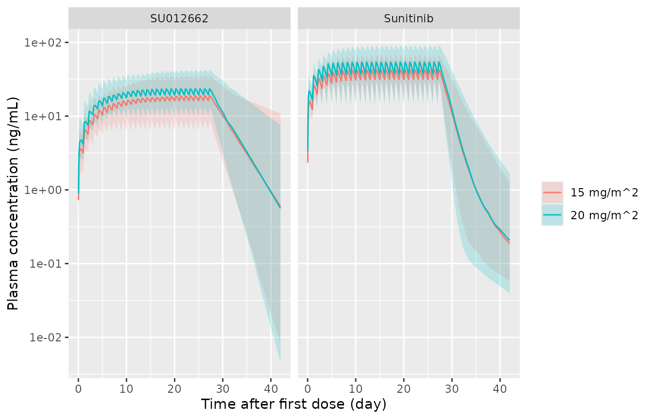

Simulated sunitinib and SU012662 plasma concentrations (median and 90% prediction interval) over the first 42-day schedule-4/2 cycle, in the spirit of Wang 2020 Figure 1a-b.

Trough concentrations on day 28 of the simulated cycle, which the trials sampled weekly:

trough <- pk_long |>
  dplyr::filter(time == 27 * 24) |>
  dplyr::group_by(analyte, treatment) |>
  dplyr::summarise(
    `Median (ng/mL)` = signif(median(conc), 3),
    `5th percentile` = signif(quantile(conc, 0.05), 3),
    `95th percentile` = signif(quantile(conc, 0.95), 3),
    .groups = "drop"
  )
knitr::kable(trough)

analyte	treatment	Median (ng/mL)	5th percentile	95th percentile
SU012662	15 mg/m^2	16.3	6.44	32.4
SU012662	20 mg/m^2	19.4	9.74	38.8
Sunitinib	15 mg/m^2	31.5	15.90	54.2
Sunitinib	20 mg/m^2	37.5	14.20	77.6

BSA effect

Wang 2020 reports that higher BSA gives greater CL/F and Vc/F, and therefore lower exposure at a fixed dose. With BSA-based dosing, the dose-normalised exposure should fall with BSA for sunitinib, because CL/F rises more than proportionally in the linear model. The typical-value CL/F across the observed BSA range:

bsa_grid <- c(0.66, 1.0, 1.47, 2.14)
data.frame(
  BSA = bsa_grid,
  `Sunitinib CL/F (L/h)` = signif(24.1 * (1 + 0.557 * (bsa_grid - 1.47)), 3),
  `SU012662 CL/F (L/h)` = signif(10.9 * (bsa_grid / 1.47)^0.843, 3),
  check.names = FALSE
) |> knitr::kable()

BSA	Sunitinib CL/F (L/h)	SU012662 CL/F (L/h)
0.66	13.2	5.55
1.00	17.8	7.88
1.47	24.1	10.90
2.14	33.1	15.00

PKNCA validation

A single dose of 20 mg/m^2 is simulated with a long sampling tail, and PKNCA computes the NCA parameters per BSA-dose arm. Because the model is linear, AUC0-inf * CL/F must return the dose (sunitinib) or 21% of the dose (SU012662) for every subject. Wang 2020 does not report an NCA table, so this closed-form identity is the quantitative gate.

sd_times <- sort(unique(c(seq(0, 24, by = 0.5), seq(24, 96, by = 2), seq(96, 2400, by = 12))))
ev_sd_pk <- make_events(cohort, sd_times, "central", n_doses = 1)
ev_sd_m <- make_events(cohort, sd_times, "central_su12662", n_doses = 1)
sd_pk <- rxode2::rxSolve(mod_pk, ev_sd_pk, keep = c("treatment", "dose_mg")) |> as.data.frame()
sd_m <- rxode2::rxSolve(mod_m, ev_sd_m, keep = c("treatment", "dose_mg")) |> as.data.frame()

run_nca <- function(sim, conc_col) {
  conc <- sim |>
    dplyr::transmute(id, time, treatment, conc = .data[[conc_col]]) |>
    dplyr::filter(!is.na(conc))
  dose <- sim |>
    dplyr::distinct(id, treatment, dose_mg) |>
    dplyr::mutate(time = 0)
  o_conc <- PKNCA::PKNCAconc(conc, conc ~ time | treatment + id, concu = "ng/mL", timeu = "h")
  o_dose <- PKNCA::PKNCAdose(dose, dose_mg ~ time | treatment + id, doseu = "mg")
  intervals <- data.frame(
    start = 0, end = Inf, cmax = TRUE, tmax = TRUE, aucinf.obs = TRUE, half.life = TRUE
  )
  PKNCA::pk.nca(PKNCA::PKNCAdata(o_conc, o_dose, intervals = intervals))
}

nca_pk <- run_nca(sd_pk, "Cc")
nca_m <- run_nca(sd_m, "Cc_su12662")
summary(nca_pk)
#>  Interval Start Interval End treatment   N Cmax (ng/mL)          Tmax (h)
#>               0          Inf 15 mg/m^2 100  17.1 [23.0] 8.00 [2.50, 26.0]
#>               0          Inf 20 mg/m^2 100  23.6 [24.8] 8.00 [3.50, 38.0]
#>  Half-life (h) AUCinf,obs (h*ng/mL)
#>     160 [1.06]           909 [34.3]
#>     160 [1.25]          1310 [33.6]
#> 
#> Caption: Cmax, AUCinf,obs: geometric mean and geometric coefficient of variation; Tmax: median and range; Half-life: arithmetic mean and standard deviation; N: number of subjects
summary(nca_m)
#>  Interval Start Interval End treatment   N Cmax (ng/mL)          Tmax (h)
#>               0          Inf 15 mg/m^2 100  3.73 [45.6] 10.8 [3.00, 34.0]
#>               0          Inf 20 mg/m^2 100  4.59 [40.8] 11.5 [3.50, 40.0]
#>  Half-life (h) AUCinf,obs (h*ng/mL)
#>    89.7 [63.2]           423 [48.3]
#>    97.5 [75.7]           554 [53.8]
#> 
#> Caption: Cmax, AUCinf,obs: geometric mean and geometric coefficient of variation; Tmax: median and range; Half-life: arithmetic mean and standard deviation; N: number of subjects

auc_check <- function(nca, sim, cl_col, frac) {
  auc <- as.data.frame(nca$result) |>
    dplyr::filter(PPTESTCD == "aucinf.obs") |>
    dplyr::select(id, treatment, auc = PPORRES)
  indiv <- sim |> dplyr::distinct(id, dose_mg, cl = .data[[cl_col]])
  dplyr::left_join(auc, indiv, by = "id") |>
    dplyr::mutate(pct_diff = 100 * (auc * cl / 1000 / (frac * dose_mg) - 1))
}
chk_pk <- auc_check(nca_pk, sd_pk, "cl", 1)
chk_m <- auc_check(nca_m, sd_m, "cl_su12662", 0.21)

rbind(
  sunitinib = quantile(chk_pk$pct_diff, c(0.05, 0.5, 0.95)),
  SU012662 = quantile(chk_m$pct_diff, c(0.05, 0.5, 0.95))
) |> signif(3)
#>                  5%      50%      95%
#> sunitinib -0.000493  0.00555  0.01230
#> SU012662  -0.015800 -0.00453 -0.00107

# Both sides use the same drawn parameters, so the difference is pure
# numerical error (trapezoidal integration and the extrapolated tail) and a
# tight bound on every subject is appropriate.
stopifnot(
  all(abs(chk_pk$pct_diff) < 0.5),
  all(abs(chk_m$pct_diff) < 0.5)
)

A typical-value check at the reference BSA (1.47 m^2, 20 mg/m^2 = 29.4 mg) compares the steady-state average concentration on day 28 against Dose / (CL/F * tau):

typ <- data.frame(id = 1, dose_m2 = 20, BSA = 1.47, dose_mg = 29.4, treatment = "typical")
ev_typ <- make_events(typ, seq(27 * 24, 28 * 24, by = 0.25), "central")
typ_pk <- rxode2::rxSolve(rxode2::zeroRe(mod_pk), ev_typ) |> as.data.frame()
#> ℹ parameter labels from comments will be replaced by 'label()'
#> ℹ omega/sigma items treated as zero: 'etalcl', 'etalvc', 'etalka'
day28 <- typ_pk[typ_pk$time >= 27 * 24 & typ_pk$time <= 28 * 24, ]
cavg_sim <- sum(diff(day28$time) * (head(day28$Cc, -1) + tail(day28$Cc, -1)) / 2) / 24
cavg_ss <- 29.4 * 1000 / (24.1 * 24)
c(simulated = cavg_sim, steady_state = cavg_ss, pct_diff = 100 * (cavg_sim / cavg_ss - 1))
#>    simulated steady_state     pct_diff 
#>  50.78170314  50.82987552  -0.09477179
# Deterministic typical-value solve: by day 28 the average concentration is
# within a fraction of a percent of steady state.
stopifnot(abs(cavg_sim / cavg_ss - 1) < 0.01)

Safety endpoints: typical-value PK-PD

Each PD model is simulated at the reference BSA (1.47 m^2) with 20 mg/m^2 once daily for 28 days and then followed off drug to day 84. A drug-free control run must hold every endpoint at its baseline, and the treated run must move each endpoint in the clinically expected direction.

pd_models <- c(
  anc = "Wang_2020_sunitinib_anc", plt = "Wang_2020_sunitinib_plt",
  wbc = "Wang_2020_sunitinib_wbc", lymphocytes = "Wang_2020_sunitinib_lymphocytes",
  hb = "Wang_2020_sunitinib_hb", alt = "Wang_2020_sunitinib_alt",
  ast = "Wang_2020_sunitinib_ast", dbp = "Wang_2020_sunitinib_dbp"
)
pd_state <- c(
  anc = "circ", plt = "circ", wbc = "circ", lymphocytes = "circ", hb = "circ",
  alt = "alt", ast = "ast", dbp = "dbp"
)
pd_label <- c(
  anc = "ANC", plt = "Platelets", wbc = "WBC", lymphocytes = "Lymphocytes",
  hb = "Hemoglobin", alt = "ALT", ast = "AST", dbp = "Diastolic BP"
)
pd_times <- seq(0, 84 * 24, by = 6)

sim_pd_typical <- function(key, dose_mg) {
  mod <- rxode2::zeroRe(readModelDb(pd_models[[key]]))
  subj <- data.frame(id = 1, dose_m2 = 20, BSA = 1.47, dose_mg = dose_mg, treatment = "typical")
  ev <- make_events(subj, pd_times, pd_state[[key]])
  s <- rxode2::rxSolve(mod, ev) |> as.data.frame()
  data.frame(endpoint = key, time = s$time, value = s[[pd_state[[key]]]], rbase = s$rbase)
}

pd_typ <- dplyr::bind_rows(lapply(names(pd_models), sim_pd_typical, dose_mg = 29.4))
#> ℹ parameter labels from comments will be replaced by 'label()'
#> ℹ omega/sigma items treated as zero: 'etalcl', 'etalvc', 'etalka', 'etalrbase', 'etalec50'
#> ℹ parameter labels from comments will be replaced by 'label()'
#> ℹ omega/sigma items treated as zero: 'etalcl', 'etalvc', 'etalka', 'etalrbase', 'etalec50'
#> ℹ parameter labels from comments will be replaced by 'label()'
#> ℹ omega/sigma items treated as zero: 'etalcl', 'etalvc', 'etalka', 'etalrbase', 'etalec50'
#> ℹ parameter labels from comments will be replaced by 'label()'
#> ℹ omega/sigma items treated as zero: 'etalcl', 'etalvc', 'etalka', 'etalrbase', 'etalec50'
#> ℹ parameter labels from comments will be replaced by 'label()'
#> ℹ omega/sigma items treated as zero: 'etalcl', 'etalvc', 'etalka', 'etalrbase', 'etalslope'
#> ℹ parameter labels from comments will be replaced by 'label()'
#> ℹ omega/sigma items treated as zero: 'etalcl', 'etalvc', 'etalka', 'etalrbase', 'etalkout', 'etalslope'
#> ℹ parameter labels from comments will be replaced by 'label()'
#> ℹ omega/sigma items treated as zero: 'etalcl', 'etalvc', 'etalka', 'etalrbase', 'etalkout', 'etalslope'
#> ℹ parameter labels from comments will be replaced by 'label()'
#> ℹ omega/sigma items treated as zero: 'etalcl', 'etalvc', 'etalka', 'etalrbase', 'etalkout', 'etalslope'
pd_ctl <- dplyr::bind_rows(lapply(names(pd_models), sim_pd_typical, dose_mg = 0))
#> ℹ parameter labels from comments will be replaced by 'label()'
#> ℹ omega/sigma items treated as zero: 'etalcl', 'etalvc', 'etalka', 'etalrbase', 'etalec50'
#> ℹ parameter labels from comments will be replaced by 'label()'
#> ℹ omega/sigma items treated as zero: 'etalcl', 'etalvc', 'etalka', 'etalrbase', 'etalec50'
#> ℹ parameter labels from comments will be replaced by 'label()'
#> ℹ omega/sigma items treated as zero: 'etalcl', 'etalvc', 'etalka', 'etalrbase', 'etalec50'
#> ℹ parameter labels from comments will be replaced by 'label()'
#> ℹ omega/sigma items treated as zero: 'etalcl', 'etalvc', 'etalka', 'etalrbase', 'etalec50'
#> ℹ parameter labels from comments will be replaced by 'label()'
#> ℹ omega/sigma items treated as zero: 'etalcl', 'etalvc', 'etalka', 'etalrbase', 'etalslope'
#> ℹ parameter labels from comments will be replaced by 'label()'
#> ℹ omega/sigma items treated as zero: 'etalcl', 'etalvc', 'etalka', 'etalrbase', 'etalkout', 'etalslope'
#> ℹ parameter labels from comments will be replaced by 'label()'
#> ℹ omega/sigma items treated as zero: 'etalcl', 'etalvc', 'etalka', 'etalrbase', 'etalkout', 'etalslope'
#> ℹ parameter labels from comments will be replaced by 'label()'
#> ℹ omega/sigma items treated as zero: 'etalcl', 'etalvc', 'etalka', 'etalrbase', 'etalkout', 'etalslope'

pd_tab <- pd_typ |>
  dplyr::group_by(endpoint) |>
  dplyr::summarise(
    baseline = dplyr::first(rbase),
    day28 = value[time == 28 * 24],
    lowest = min(value),
    highest = max(value),
    day84 = value[time == 84 * 24],
    .groups = "drop"
  ) |>
  dplyr::mutate(
    extreme = ifelse(endpoint %in% c("alt", "ast", "dbp"), highest, lowest),
    pct_day28 = 100 * (day28 / baseline - 1)
  ) |>
  dplyr::select(-lowest, -highest)
pd_tab |>
  dplyr::mutate(endpoint = pd_label[endpoint], dplyr::across(where(is.numeric), ~ signif(.x, 3))) |>
  dplyr::rename(
    Endpoint = endpoint, Baseline = baseline, `Day 28` = day28,
    `Nadir or peak` = extreme, `Day 84` = day84, `% change day 28` = pct_day28
  ) |>
  knitr::kable()

Endpoint	Baseline	Day 28	Day 84	Nadir or peak	% change day 28
ALT	26.5	33.70	26.50	33.70	27.0000
ANC	3.7	1.57	3.44	1.57	-57.5000
AST	26.2	33.00	26.20	36.60	26.0000
Diastolic BP	65.9	73.40	65.90	73.50	11.3000
Hemoglobin	13.0	13.00	12.80	12.80	-0.0922
Lymphocytes	1.5	1.50	1.33	1.33	-0.2930
Platelets	242.0	163.00	239.00	163.00	-32.7000
WBC	6.1	3.88	5.71	3.86	-36.3000

ctl_dev <- pd_ctl |>
  dplyr::group_by(endpoint) |>
  dplyr::summarise(max_rel_dev = max(abs(value / rbase - 1)), .groups = "drop")
stopifnot(all(ctl_dev$max_rel_dev < 1e-6))

falls <- c("anc", "plt", "wbc", "lymphocytes", "hb")
rises <- c("alt", "ast", "dbp")
stopifnot(
  all(pd_tab$pct_day28[pd_tab$endpoint %in% falls] < 0),
  all(pd_tab$pct_day28[pd_tab$endpoint %in% rises] > 0)
)

pd_typ |>
  dplyr::mutate(pct = 100 * value / rbase, endpoint = pd_label[endpoint]) |>
  ggplot(aes(time / 24, pct)) +
  geom_line() +
  geom_vline(xintercept = 28, linetype = 2, colour = "grey50") +
  facet_wrap(~endpoint, scales = "free_y", ncol = 4) +
  labs(x = "Time after first dose (day)", y = "Percent of baseline")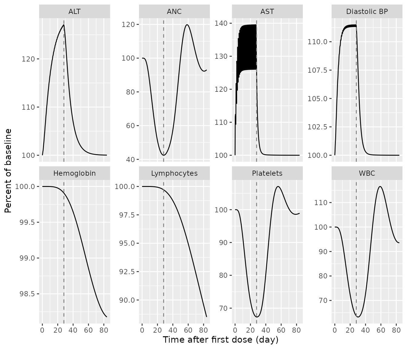

Typical-value time course of each safety endpoint (percent of baseline) for a patient with BSA 1.47 m^2 receiving sunitinib 20 mg/m^2 once daily on days 1-28.

Safety endpoints: stochastic simulation

The 20 mg/m^2 arm of the virtual cohort is run through each PD model with between-subject variability on both the PK layer and the PD parameters, in the spirit of the Wang 2020 Figure 1c-j VPCs.

arm20 <- cohort[cohort$dose_m2 == 20, ]
sim_pd_vpc <- function(key) {
  mod <- readModelDb(pd_models[[key]])
  ev <- make_events(arm20, seq(0, 84 * 24, by = 12), pd_state[[key]])
  s <- rxode2::rxSolve(mod, ev) |> as.data.frame()
  data.frame(endpoint = key, id = s$id, time = s$time, value = s[[pd_state[[key]]]])
}
pd_vpc <- dplyr::bind_rows(lapply(names(pd_models), sim_pd_vpc))
#> ℹ parameter labels from comments will be replaced by 'label()'
#> ℹ parameter labels from comments will be replaced by 'label()'
#> ℹ parameter labels from comments will be replaced by 'label()'
#> ℹ parameter labels from comments will be replaced by 'label()'
#> ℹ parameter labels from comments will be replaced by 'label()'
#> ℹ parameter labels from comments will be replaced by 'label()'
#> ℹ parameter labels from comments will be replaced by 'label()'
#> ℹ parameter labels from comments will be replaced by 'label()'
pd_vpc_sum <- pd_vpc |>
  dplyr::group_by(endpoint, time) |>
  dplyr::summarise(
    q05 = quantile(value, 0.05), q50 = median(value), q95 = quantile(value, 0.95),
    .groups = "drop"
  ) |>
  dplyr::mutate(endpoint = pd_label[endpoint])

ggplot(pd_vpc_sum, aes(time / 24, q50)) +
  geom_ribbon(aes(ymin = q05, ymax = q95), alpha = 0.25) +
  geom_line() +
  geom_vline(xintercept = 28, linetype = 2, colour = "grey50") +
  facet_wrap(~endpoint, scales = "free_y", ncol = 4) +
  labs(x = "Time after first dose (day)", y = "Endpoint value (units as in Table 4)")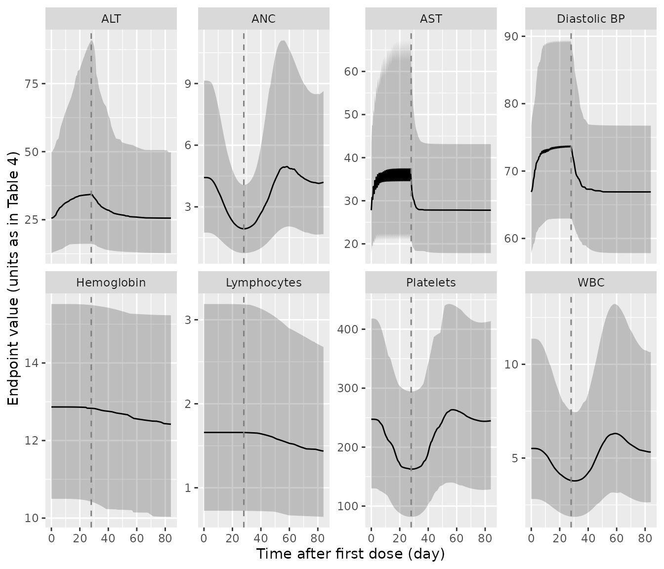

Simulated safety endpoints (median and 90% prediction interval) for 100 virtual patients receiving sunitinib 20 mg/m^2 once daily on days 1-28.

Hemoglobin and lymphocyte count barely move within one 28-day course because their mean transit times are long (1370 h and 1990 h, about 57 and 83 days), so the stochastic check below is restricted to the six endpoints with a material day-28 change; the typical-value checks above cover all eight.

# Median day-28 change must agree in direction with the typical-value run,
# with a margin well clear of zero.
med28 <- pd_vpc |>
  dplyr::group_by(endpoint, id) |>
  dplyr::summarise(pct = 100 * (value[time == 28 * 24] / value[time == 0] - 1), .groups = "drop") |>
  dplyr::group_by(endpoint) |>
  dplyr::summarise(median_pct = median(pct), .groups = "drop")
knitr::kable(dplyr::mutate(med28, endpoint = pd_label[endpoint], median_pct = signif(median_pct, 3)))

endpoint	median_pct
ALT	27.800
ANC	-57.100
AST	25.700
Diastolic BP	9.520
Hemoglobin	-0.089
Lymphocytes	-0.281
Platelets	-30.300
WBC	-35.500

stopifnot(
  all(med28$median_pct[med28$endpoint %in% c("anc", "plt", "wbc")] < -10),
  all(med28$median_pct[med28$endpoint %in% rises] > 3)
)

The linear inhibition of kout used for ALT and AST (see Assumptions) turns the loss rate negative whenever kPD * C exceeds 1. The share of simulated subjects in which that happens at any time during the 20 mg/m^2 course:

flip_share <- function(key) {
  mod <- readModelDb(pd_models[[key]])
  ev <- make_events(arm20, seq(0, 28 * 24, by = 2), pd_state[[key]])
  s <- rxode2::rxSolve(mod, ev) |> as.data.frame()
  per_id <- tapply(s$slope * s$Cc, s$id, max)
  mean(per_id > 1)
}
flip <- c(ALT = flip_share("alt"), AST = flip_share("ast"))
round(100 * flip, 1)
#> ALT AST 
#>  12   0
# The typical subject is far from the sign change (ALT kPD * C is about 0.2-0.3).
stopifnot(all(flip < 0.2))

Assumptions and deviations

• Two separate PK models. Wang 2020 fitted sunitinib and SU012662 as two independent two-compartment models, each with its own absorption rate and lag time, rather than a joint parent-metabolite model. They are packaged as two files. The SU012662 model receives 21% of the sunitinib dose into its depot (fdepot fixed to 0.21), the conversion the authors state they assumed. The paper does not say whether a molecular-weight correction was applied; the fraction is applied to the sunitinib dose in mg as printed.
• BSA coefficients. The BSA effects use the values printed in the Results equations (0.557, 1.47, 0.843, 1.72); Table 3 rounds the first and third to 0.56 and 0.84.
• IIV scale. Tables 3 and 4 print between-subject variability as a percentage. It is read as a log-normal CV and converted with omega^2 = log(1 + CV^2). If the authors instead reported 100 * sqrt(omega^2) the variances would be larger, most visibly for the parameters printed above 100% (for example AST kout at 435%, lymphocyte EC50 at 404%).
• Residual error. Sigma is printed as a percentage for every endpoint and is encoded as a proportional error.
• PD equations are not printed in Wang 2020. The paper names each model type and cites Khosravan 2016 for the structures. Khosravan 2016 Figure 5 fixes the transit/feedback layout (proliferating pool, three transit compartments, circulating pool, Kprol = Ktr = Kcirc, feedback (Circ0/Circ)^gamma) and the indirect-response layout; its supplement gives no equations either. The following choices follow standard practice for these model types:
  • Ktr = 4 / MTT, the Friberg 2002 definition of mean transit time for three transit compartments.
  • The Emax effect inhibits proliferation as (1 - Edrug) with Edrug = Emax * C^GAM / (EC50^GAM + C^GAM).
  • The first-order kPD (mL/ng) effects are linear in the sunitinib concentration: kprol * (1 - kPD * C) for hemoglobin, kout * (1 - kPD * C) for ALT and AST, and kin * (1 + kPD * C) for diastolic BP. The directions follow the clinical effects (falling hemoglobin, rising transaminases and blood pressure).
• Linear inhibition of kout can change sign. With kout * (1 - kPD * C), a subject whose kPD * C exceeds 1 has a negative loss rate while on drug, and ALT or AST then grows until dosing stops. At 20 mg/m^2 this needs a kPD several-fold above the typical value. It never happens for AST, whose kPD variability is small, but the wide ALT kPD variability (97.9% CV) puts a minority of simulated ALT subjects past it (the share is computed above). Those subjects show an unbounded on-treatment rise that the paper’s concentration range may not have exercised; a reciprocal form such as kout / (1 + kPD * C) would avoid it, but the paper does not print the equation, so the linear form is kept.
• Table 4 typographical issues. Hemoglobin BASE is printed in “10^9/L”; the value 13.0 is a hemoglobin concentration in g/dL. The bootstrap interval printed for ALT kout (0.00131-0.00195) does not contain its own median (0.00553); the model uses the final estimate 0.00559. The lymphocyte EC50 and omega bootstrap intervals are garbled in print; only the final estimates are used.
• Sequential PK-PD. In each PD file the sunitinib PK parameters and their variances are wrapped in fixed(). In the paper the PD fits used the individual PK predictions; simulating from these files draws new PK random effects instead.
• Virtual cohort. BSA is drawn from a log-normal distribution with median 1.47 m^2 and a log-scale SD of 0.3, redrawn into the observed range; the paper reports only the median and range. Doses are not rounded to capsule strengths.
• No published NCA or PD summary to reproduce. Wang 2020 reports model parameters, VPC figures and adverse-event incidences, but no NCA table or numeric PD simulations, so validation relies on closed-form identities and the direction of each drug effect.