Benznidazole (Soy 2015)
Source:vignettes/articles/Soy_2015_benznidazole.Rmd
Soy_2015_benznidazole.RmdModel and source
- Citation: Soy D, Aldasoro E, Guerrero L, Posada E, Serret N, Mejia T, Urbina JA, Gascon J. Population pharmacokinetics of benznidazole in adult patients with Chagas disease. Antimicrobial Agents and Chemotherapy. 2015;59(6):3342-3349. doi:10.1128/AAC.05018-14.
- Description: One-compartment population PK model with first-order absorption and first-order elimination for oral benznidazole in adult patients with chronic Chagas disease (Soy 2015; CINEBENZ trial, n = 39 index plus n = 10 external validation). Apparent clearance CL/F = 1.73 L/h, apparent volume of distribution V/F = 89.6 L, and absorption rate constant Ka = 1.15 1/h fixed from the literature (Raaflaub & Ziegler 1979). Inter-individual variability is on CL/F (33.4% CV) and V/F (68.8% CV); inter-occasion variability is on CL/F (29.5% CV), folded into the CL/F eta as BSV-equivalent for forward simulation. Residual error is combined additive (0.57 mg/L) plus proportional (19.53% CV). No demographic or biological covariates were retained in the final model.
- Article: https://doi.org/10.1128/AAC.05018-14
- Trial registry: EudraCT 2011-002900-34, ClinicalTrials.gov NCT01755403 (CINEBENZ).
Population
Soy 2015 (CINEBENZ) enrolled 52 adult patients with chronic Chagas disease at the Tropical Medicine Unit of the Hospital Clinic of Barcelona. After dropouts and treatment discontinuations, the popPK index data set comprised 358 plasma samples from 39 patients (26 female / 13 male; mean age 37.15 years, range 19-55; mean total body weight 70.55 kg, range 43-100; 96% originally from Bolivia). A separate validation cohort of 10 patients (96 samples) was used for external predictive-performance assessment but not for parameter estimation. Treatment was oral benznidazole 2.5 mg/kg every 12 hours for 8 weeks (maximum 400 mg/day; Abarax, Elea Laboratory, Argentina). Median drug adherence across the cohort was 99.2%. Baseline demographics are in Soy 2015 Table 1.
The same information is available programmatically via the model’s
population metadata
(readModelDb("Soy_2015_benznidazole")()$population).
Source trace
The per-parameter origin is recorded inline next to each
ini() entry in
inst/modeldb/specificDrugs/Soy_2015_benznidazole.R. The
table below collects them in one place for review.
| Equation / parameter | Value | Source location |
|---|---|---|
lka (= log(1.15)) |
Ka = 1.15 1/h, FIXED | Soy 2015 Table 2 (“Ka 1.15 (fixed)”) and Discussion paragraph 2 (“Ka was set to a fixed value obtained from the literature (8)”). Source 8 is Raaflaub & Ziegler (1979). |
lcl (= log(1.73)) |
CL/F = 1.73 L/h | Soy 2015 Table 2 (CL/F final estimate). |
lvc (= log(89.6)) |
V/F = 89.6 L | Soy 2015 Table 2 (V/F final estimate). |
etalcl variance |
log(1 + 0.334^2) + log(1 + 0.295^2) | Soy 2015 Table 2: IIV CL/F = 33.4% CV and IOV CL/F = 29.5% CV; IOV folded into CL/F BSV-equivalent eta for forward simulation. |
etalvc variance |
log(1 + 0.688^2) | Soy 2015 Table 2 (IIV V/F = 68.8% CV). |
addSd |
0.57 mg/L | Soy 2015 Table 2 (sigma^2_1 additive residual SD). |
propSd |
0.1953 (fraction CV) | Soy 2015 Table 2 (sigma^2_2 proportional residual error, 19.53% CV). |
d/dt(depot) and d/dt(central)
|
one-compartment with first-order absorption and elimination | Soy 2015 Results, “Population pharmacokinetic model” paragraph; Discussion paragraph 2 (“open one-compartment PK model with first-order absorption and elimination”). |
Virtual cohort
Original observed concentrations are not publicly available. The cohort below matches the index data set demographics (n = 39, mean weight 70.55 kg, 71% female) and the published dosing regimen (2.5 mg/kg every 12 hours for 60 days), with simulated plasma samples on a regular grid.
set.seed(20250602)

n_subjects <- 200
dose_interval_h <- 12       # q12h
treatment_days <- 60
n_doses <- treatment_days * 24 / dose_interval_h

# Use a log-normal weight distribution that approximately reproduces the
# Soy 2015 Table 1 mean 70.55 kg and SD 14.5 kg in the index cohort, with
# the observed 43-100 kg range respected by truncation.
wt_meanlog <- log(70.55^2 / sqrt(70.55^2 + 14.5^2))
wt_sdlog   <- sqrt(log(1 + (14.5 / 70.55)^2))
wt_kg <- pmin(100, pmax(43, rlnorm(n_subjects, wt_meanlog, wt_sdlog)))

cohort <- tibble::tibble(
  id = seq_len(n_subjects),
  WT = wt_kg
) |>
  mutate(amt_mg = 2.5 * WT)

# Dosing rows (evid = 1) every 12 hours for 60 days, plus a dense
# observation grid for VPC over the first 24 hours after the first
# dose and over the last steady-state interval.
dose_rows <- cohort |>
  tidyr::expand_grid(dose_idx = seq_len(n_doses)) |>
  mutate(
    time = (dose_idx - 1L) * dose_interval_h,
    amt  = amt_mg,
    evid = 1L,
    cmt  = "depot"
  ) |>
  select(id, time, amt, evid, cmt)

obs_grid_day1 <- seq(0, 24, by = 0.5)
obs_grid_ss <- seq(treatment_days * 24 - 24, treatment_days * 24, by = 0.5)

obs_rows <- cohort |>
  tidyr::expand_grid(time = sort(unique(c(obs_grid_day1, obs_grid_ss)))) |>
  mutate(amt = NA_real_, evid = 0L, cmt = "central") |>
  select(id, time, amt, evid, cmt)

events <- bind_rows(dose_rows, obs_rows) |>
  arrange(id, time, desc(evid))

# Required by Soy 2015 model: no covariates needed in events (final
# model has no covariate effects). WT is used by the cohort tibble
# only to scale the mg/kg dose.

stopifnot(!anyDuplicated(unique(events[, c("id", "time", "evid")])))
Simulation
mod <- readModelDb("Soy_2015_benznidazole")
sim <- rxode2::rxSolve(mod, events = events) |> as.data.frame()
#> ℹ parameter labels from comments will be replaced by 'label()'
Replicate published figures
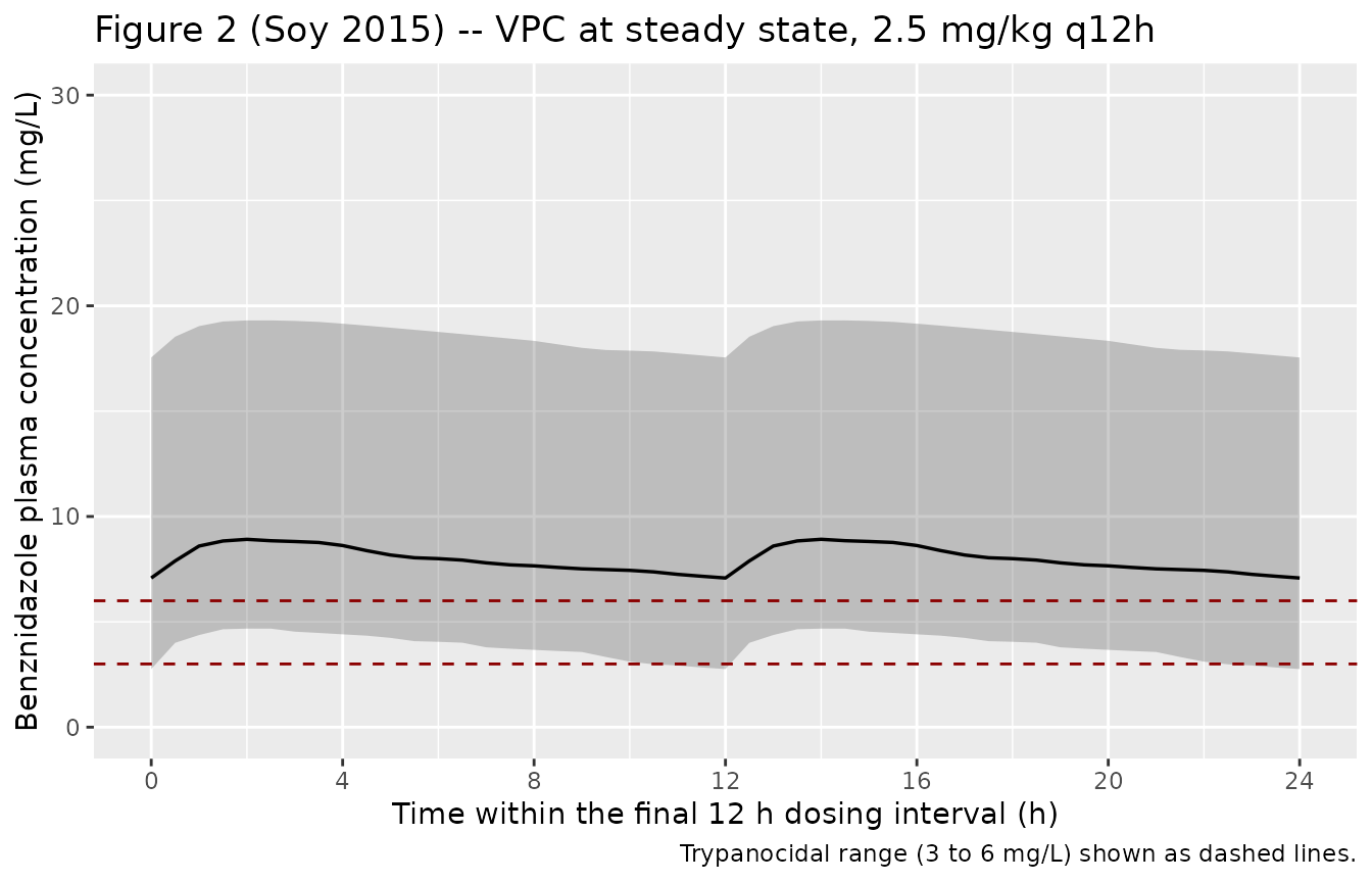
# Replicates Figure 2 of Soy 2015: VPC at steady state (5th, 50th,
# 95th percentiles). Soy 2015 Figure 2 plots the full observation
# horizon; here we show the final 24 h interval at steady state.
sim_ss <- sim |>
  filter(time >= treatment_days * 24 - 24, time <= treatment_days * 24) |>
  mutate(time_in_interval = time - (treatment_days * 24 - 24))

vpc_df <- sim_ss |>
  group_by(time_in_interval) |>
  summarise(
    Q05 = quantile(Cc, 0.05, na.rm = TRUE),
    Q50 = quantile(Cc, 0.50, na.rm = TRUE),
    Q95 = quantile(Cc, 0.95, na.rm = TRUE),
    .groups = "drop"
  )

ggplot(vpc_df, aes(time_in_interval, Q50)) +
  geom_ribbon(aes(ymin = Q05, ymax = Q95), alpha = 0.25) +
  geom_line(linewidth = 0.6) +
  geom_hline(yintercept = c(3, 6), linetype = "dashed", colour = "darkred") +
  scale_x_continuous(breaks = seq(0, 24, by = 4)) +
  scale_y_continuous(limits = c(0, 30)) +
  labs(
    x = "Time within the final 12 h dosing interval (h)",
    y = "Benznidazole plasma concentration (mg/L)",
    title = "Figure 2 (Soy 2015) -- VPC at steady state, 2.5 mg/kg q12h",
    caption = "Trypanocidal range (3 to 6 mg/L) shown as dashed lines."
  )
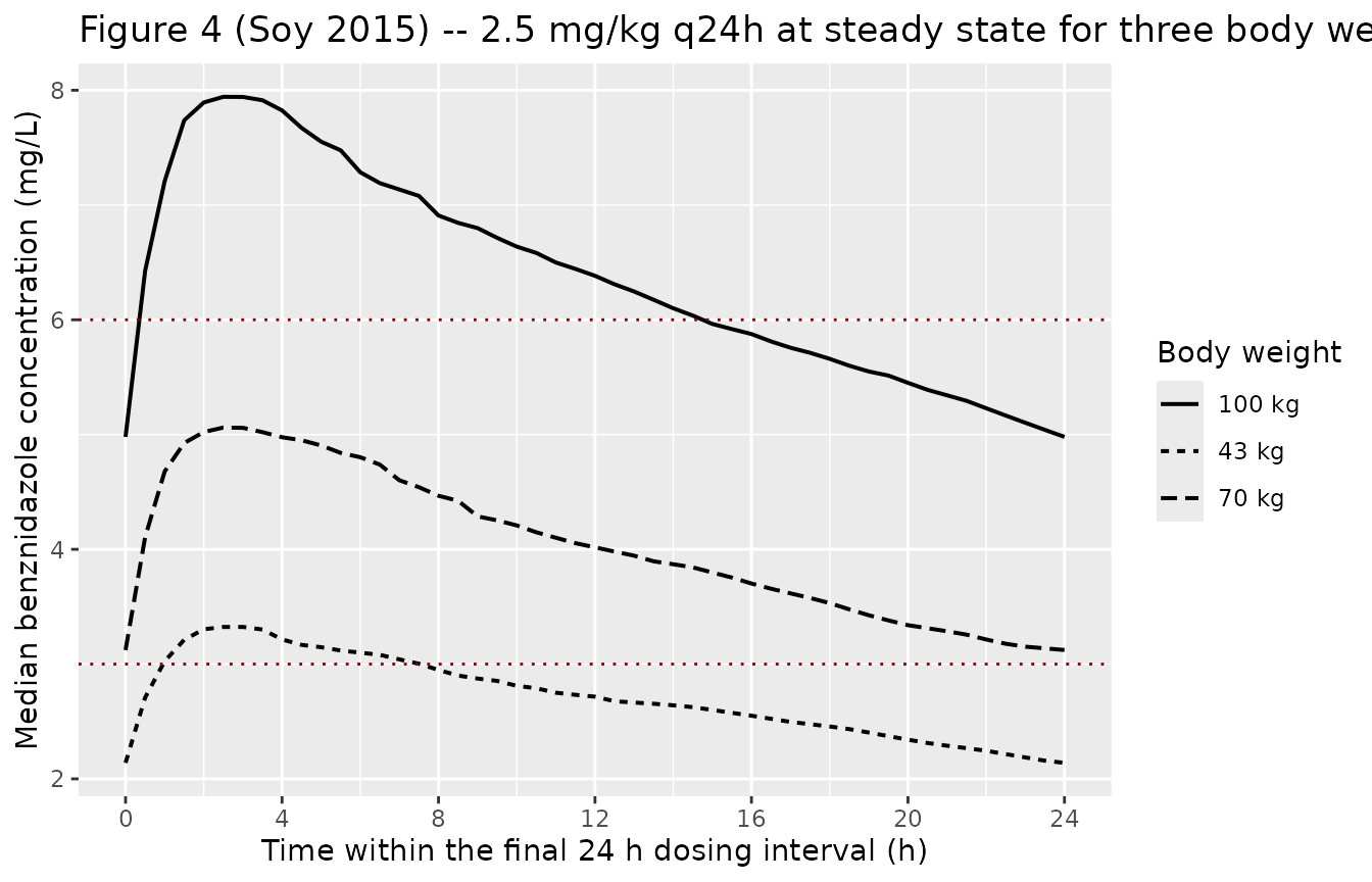
# Replicates Figure 4 of Soy 2015: median steady-state concentration
# vs time within a dosing interval at 2.5 mg/kg q24h for three body
# weights (43, 70, 100 kg).
make_cohort_q24 <- function(weight_kg, id_offset, n = 200) {
  tibble::tibble(
    id = id_offset + seq_len(n),
    WT = weight_kg,
    amt_mg = 2.5 * weight_kg
  )
}

dose_q24 <- 24
ndose_q24 <- treatment_days

build_events_q24 <- function(cohort_df) {
  doses <- cohort_df |>
    tidyr::expand_grid(dose_idx = seq_len(ndose_q24)) |>
    mutate(time = (dose_idx - 1L) * dose_q24, amt = amt_mg,
           evid = 1L, cmt = "depot") |>
    select(id, time, amt, evid, cmt)
  obs <- cohort_df |>
    tidyr::expand_grid(time = seq(treatment_days * 24 - 24, treatment_days * 24,
                                   by = 0.5)) |>
    mutate(amt = NA_real_, evid = 0L, cmt = "central") |>
    select(id, time, amt, evid, cmt)
  bind_rows(doses, obs) |> arrange(id, time, desc(evid))
}

cohorts_q24 <- bind_rows(
  make_cohort_q24( 43, id_offset =    0L) |> mutate(cohort = "43 kg"),
  make_cohort_q24( 70, id_offset =  200L) |> mutate(cohort = "70 kg"),
  make_cohort_q24(100, id_offset =  400L) |> mutate(cohort = "100 kg")
)
events_q24 <- build_events_q24(cohorts_q24)
stopifnot(!anyDuplicated(unique(events_q24[, c("id", "time", "evid")])))

# Carry cohort label through rxSolve via keep.
events_q24_keep <- events_q24 |>
  left_join(cohorts_q24 |> select(id, cohort), by = "id")

sim_q24 <- rxode2::rxSolve(mod, events = events_q24_keep,
                           keep = c("cohort")) |>
  as.data.frame()
#> ℹ parameter labels from comments will be replaced by 'label()'

sim_q24_ss <- sim_q24 |>
  filter(time >= treatment_days * 24 - 24, time <= treatment_days * 24) |>
  mutate(time_in_interval = time - (treatment_days * 24 - 24))

median_q24 <- sim_q24_ss |>
  group_by(cohort, time_in_interval) |>
  summarise(median_Cc = median(Cc, na.rm = TRUE), .groups = "drop")

ggplot(median_q24, aes(time_in_interval, median_Cc, linetype = cohort)) +
  geom_line(linewidth = 0.7) +
  geom_hline(yintercept = c(3, 6), linetype = "dotted", colour = "darkred") +
  scale_x_continuous(breaks = seq(0, 24, by = 4)) +
  labs(
    x = "Time within the final 24 h dosing interval (h)",
    y = "Median benznidazole concentration (mg/L)",
    title = "Figure 4 (Soy 2015) -- 2.5 mg/kg q24h at steady state for three body weights",
    linetype = "Body weight"
  )
PKNCA validation
The paper does not report a classical Cmax / AUC / Cmin table at
steady state, but it does report a terminal half-life of “about 36 h”
(Discussion paragraph 4). PKNCA’s half.life on the final
steady-state dosing interval provides the matching comparison; Cmax,
Tmax, and AUC0-tau at steady state are additionally computed for
completeness.
conc_for_nca <- sim |>
  filter(time >= treatment_days * 24 - dose_interval_h,
         time <= treatment_days * 24) |>
  mutate(time_in_interval = time - (treatment_days * 24 - dose_interval_h)) |>
  filter(!is.na(Cc), Cc > 0) |>
  mutate(treatment = "2.5 mg/kg q12h") |>
  select(id, time = time_in_interval, Cc, treatment)

dose_for_nca <- cohort |>
  mutate(time = 0, amt = amt_mg, treatment = "2.5 mg/kg q12h") |>
  select(id, time, amt, treatment)

conc_obj <- PKNCA::PKNCAconc(conc_for_nca, Cc ~ time | treatment + id,
                             concu = "mg/L", timeu = "h")
dose_obj <- PKNCA::PKNCAdose(dose_for_nca, amt ~ time | treatment + id,
                             doseu = "mg")

intervals <- data.frame(
  start    = 0,
  end      = dose_interval_h,
  cmax     = TRUE,
  tmax     = TRUE,
  cmin     = TRUE,
  auclast  = TRUE,
  half.life = TRUE
)

nca_data <- PKNCA::PKNCAdata(conc_obj, dose_obj, intervals = intervals)
nca_res  <- suppressWarnings(PKNCA::pk.nca(nca_data))

nca_tbl <- as.data.frame(nca_res$result) |>
  filter(PPTESTCD %in% c("cmax", "tmax", "cmin", "auclast", "half.life")) |>
  group_by(PPTESTCD) |>
  summarise(
    median = median(PPORRES, na.rm = TRUE),
    q05    = quantile(PPORRES, 0.05, na.rm = TRUE),
    q95    = quantile(PPORRES, 0.95, na.rm = TRUE),
    .groups = "drop"
  )

knitr::kable(
  nca_tbl,
  digits = 3,
  caption = paste(
    "Simulated steady-state NCA over the final 12 h interval at",
    "2.5 mg/kg q12h (n =", n_subjects, "virtual subjects).",
    "Concentrations in mg/L, time in h, AUC in mg*h/L."
  )
)| PPTESTCD | median | q05 | q95 |
|---|---|---|---|
| auclast | 94.689 | 48.128 | 223.059 |
| cmax | 8.918 | 4.678 | 19.308 |
| cmin | 7.080 | 2.758 | 17.549 |
| half.life | 33.238 | 8.706 | 119.950 |
| tmax | 2.000 | 2.000 | 2.500 |
Comparison against published trough concentrations
Soy 2015 Table 3 reports the simulated steady-state trough concentration (at 12 h within the dosing interval) for the standard 2.5 mg/kg q12h regimen as median 7.53 mg/L (90% CI 2.81 to 17.48) for an average 70 kg patient. The terminal half-life is reported as “about 36 h” in the Discussion.
trough_idx <- which.min(abs(median_q24$time_in_interval - 24))   # not used directly
trough_q12 <- sim_ss |>
  filter(abs(time_in_interval - dose_interval_h) < 1e-6) |>
  summarise(
    median = median(Cc, na.rm = TRUE),
    q05    = quantile(Cc, 0.05, na.rm = TRUE),
    q95    = quantile(Cc, 0.95, na.rm = TRUE)
  )

half_life_sim <- nca_tbl |> filter(PPTESTCD == "half.life") |>
  pull(median)

comparison <- tibble::tibble(
  Quantity = c(
    "Trough at 12 h, 2.5 mg/kg q12h (mg/L; median, 90% CI)",
    "Terminal half-life (h)"
  ),
  `Soy 2015 (paper)` = c(
    "7.53 (2.81 to 17.48) for 70 kg",
    "~36"
  ),
  `Simulated` = c(
    sprintf("%.2f (%.2f to %.2f)", trough_q12$median,
            trough_q12$q05, trough_q12$q95),
    sprintf("%.1f", half_life_sim)
  )
)

knitr::kable(comparison, caption = "Side-by-side comparison.")| Quantity | Soy 2015 (paper) | Simulated |
|---|---|---|
| Trough at 12 h, 2.5 mg/kg q12h (mg/L; median, 90% CI) | 7.53 (2.81 to 17.48) for 70 kg | 7.08 (2.76 to 17.55) |
| Terminal half-life (h) | ~36 | 33.2 |
The deterministic half-life implied by
log(2) / (CL/F / V/F) = log(2) / (1.73 / 89.6)
is about 35.9 h, matching the paper’s reported ~36 h. The simulated
steady-state trough distribution at 2.5 mg/kg q12h brackets the paper’s
reported median trough of 7.53 mg/L for a 70 kg patient.
Assumptions and deviations
-
No covariates retained. The paper screened age,
gender, total body weight, body mass index, creatinine clearance, total
serum proteins, total bilirubin, and hematocrit and did not retain any
in the final model (Soy 2015 Results, covariate model selection
paragraph). The packaged model has no covariate effects; the screened
covariates are documented in
covariatesDataExcludedfor provenance only. - Allometric / WT-popPK model NOT packaged. Soy 2015 also reported an exploratory model that added body-weight allometric scaling (CL exponent 0.75, V exponent 1 fixed) to the same one-compartment structure (WT-popPK; Methods “Influence of body weight on dosage”). The authors reported that this model did not improve fit and that the parameter estimates were essentially unchanged (CL/F = 1.75 L/h, V/F = 95.3 L, IIV CL/F = 34.1% CV, IIV V/F = 77.3% CV, IOV CL/F = 30% CV). Per the replicate-author-structure policy, sensitivity analyses that the authors did not adopt as final are not packaged as separate model files. The simulated body-weight stratification in Figure 4 above therefore reflects only the dosing-driven scaling (mg/kg), not an allometric structural effect.
-
IOV folded into BSV-equivalent eta. The paper
reports IOV on CL/F (29.5% CV) separately from IIV on CL/F (33.4% CV).
nlmixr2lib has no idiomatic encoding for per-occasion variability
independent of between-subject variability, so the IOV variance is added
to
etalclfor forward simulation (total CL/F variance =log(1 + 0.334^2) + log(1 + 0.295^2), geometric CV ~= 45.6%). The Denti_2018_levofloxacin model uses the same approach and cites the same nlmixr2lib precedent. - Virtual cohort weight distribution. Soy 2015 Table 1 reports mean 70.55 kg and SD 14.5 kg in the index data set; the virtual cohort draws from a log-normal distribution with those moments, truncated to the observed 43-100 kg range. Sex, ethnicity, and clinical laboratory covariates are not used by the model and are not simulated.
-
Validation cohort not simulated. The 10-patient
external validation cohort (Table 1 right column) was used by the
authors only for the PRED / IPRED bias-and-precision assessment shown in
Figure 3; no separate model is fit to it. The model file documents both
cohorts in
population$validation_cohortfor provenance. - Ka uncertainty. Ka is FIXED at 1.15 1/h from the literature (Raaflaub & Ziegler 1979, ref 8 in Soy 2015); the available trial sampling did not support its estimation (Soy 2015 Results, “Population pharmacokinetic model” paragraph).
- Residual error CV%. The Soy 2015 Results text quotes the proportional residual error as 19.1% CV; Soy 2015 Table 2 reports 19.53% CV. The Table 2 value is used here as the authoritative reported estimate.