Polymyxin B (Tang 2023)
Source:vignettes/articles/Tang_2023_polymyxinB.Rmd
Tang_2023_polymyxinB.RmdModel and source
- Citation: Tang T, Li Y, Xu P, Zhong Y, Yang M, Ma W, Xiang D, Zhang B, Zhou Y. Optimization of polymyxin B regimens for the treatment of carbapenem-resistant organism nosocomial pneumonia: a real-world prospective study. Crit Care. 2023;27:164. doi:10.1186/s13054-023-04448-z. PMCID PMC10142183.
- Description: Two-compartment intravenous population PK model for polymyxin B in critically ill adults with carbapenem-resistant organism nosocomial pneumonia, developed from a prospective Chinese ICU cohort (Tang 2023). No covariate was retained. Inter-individual variability on CL and Vc only, with a 100% CL-Vc correlation encoded as a single shared random effect scaled onto Vc; variability on CLd and Vp was held at zero. Proportional residual error.
- Article: Crit Care. 2023;27:164
Population
Tang 2023 is a prospective study run in two intensive care units of the Second Xiangya Hospital of Central South University (Changsha, China) between January 2020 and December 2021. It enrolled 105 critically ill adults with hospital-acquired pneumonia caused by carbapenem-resistant organisms (CRO) who received intravenous polymyxin B for more than 3 days. Patients on renal replacement therapy were excluded.
The cohort (Table 1) was 72.4% male, with median age 65 years (IQR 55-76), weight 55.0 kg (IQR 50.0-65.0), albumin 30.7 g/L and Cockcroft-Gault creatinine clearance 72.2 mL/min (IQR 50.5-111.5). Median APACHE II score was 18; 77.1% were mechanically ventilated and 39.0% were septic. The pathogens were carbapenem-resistant Acinetobacter baumannii (81.9%), Klebsiella pneumoniae (40.0%) and Pseudomonas aeruginosa (21.9%), and every patient received polymyxin B in combination with another antimicrobial.
Polymyxin B was given as a 100-200 mg loading dose (median 100 mg) followed by 40-100 mg every 12 h, infused over at least 1 h; the median daily dose was 150 mg (2.3 mg/kg/day). Two to six plasma samples per patient (295 in total) were drawn around the seventh dose – immediately before it and at 0, 1, 2, 4, 6, 8 and 10 h after the end of infusion – and total polymyxin B (B1 + B2) was measured by HPLC-MS/MS.
The same information is available programmatically via the model’s
population metadata
(readModelDb("Tang_2023_polymyxinB")()$population).
Source trace
| Model element | Value | Source location |
|---|---|---|
| Two-compartment disposition, IV infusion into central | – | Results, “Population PK Model and polymyxin B exposure”: “A two-compartment model fully described the data” |
| No covariates | – | Same paragraph: “no covariate was statistically significant to PK parameters” |
lcl = log(1.56) |
CL 1.56 L/h | Table 2, row “CL (L/h)” (SE 4.50%); final-model equation
CL = 1.56 * exp(eta_CL)
|
lvc = log(12.5) |
Vc 12.5 L | Table 2, row “Vc (L)” (SE 5.67%);
Vc = 12.5 * exp(eta_Vc)
|
lq = log(2.41) |
CLd 2.41 L/h | Table 2, row “CLd (L/h)” (SE 11.8%); CLd = 2.41
|
lvp = log(29.9) |
Vp 29.9 L | Table 2, row “Vp (L)” (SE 17.3%); Vp = 29.9
|
etalcl = 0.394^2 |
omega CL 39.4% | Table 2, row “omega CL” (SE 6.4%) |
vc_eta_scale = 0.286 / 0.394 |
0.7259 | Derived from Table 2 rows “omega Vc” = 28.6% and “omega CL*Vc” = 100 (the correlation) |
etalq, etalvp = 0 |
– | Results: “the inter-individual variability (IIV) of CLd and Vp were fixed 0” (shrinkage > 50%) |
propSd = 0.2786 |
27.86% | Table 2, row “Proportional residual (%)” (SE 9.11%) |
Virtual cohort and simulation design
The paper simulated five regimens, each a loading dose followed by a maintenance dose every 12 h, infused over 2 h (Methods, “Monte Carlo simulations of dosage regimens”; Figure 6 legend). The model has no covariates, so the virtual patients differ only in their random effects.
mod <- readModelDb("Tang_2023_polymyxinB")

regimens <- tibble::tribble(
  ~regimen,        ~ld, ~md,
  "100 + 50 mg",   100,  50,
  "150 + 75 mg",   150,  75,
  "150 + 100 mg",  150, 100,
  "200 + 100 mg",  200, 100,
  "200 + 150 mg",  200, 150
) |>
  dplyr::mutate(regimen = factor(regimen, levels = regimen))

# Doses at 0, 12, ..., 84 h cover days 1-4; the first is the loading dose.
make_doses <- function(ids, ld, md, dur) {
  tidyr::expand_grid(id = ids, time = seq(0, 84, by = 12)) |>
    dplyr::mutate(amt = ifelse(time == 0, ld, md), dur = dur,
                  evid = 1L, cmt = "central")
}

make_obs <- function(ids, times) {
  tidyr::expand_grid(id = ids, time = times) |>
    dplyr::mutate(amt = NA_real_, dur = NA_real_, evid = 0L, cmt = "central")
}

n_per_arm <- 200L  # cap: never more than 200 participants per arm
rxode2::rxSetSeed(20231027)
Typical-value profiles
mod_tv <- rxode2::zeroRe(mod)
#> ℹ parameter labels from comments will be replaced by 'label()'

tv_events <- dplyr::bind_rows(
  lapply(seq_len(nrow(regimens)), function(i) {
    dplyr::bind_rows(
      make_doses(i, regimens$ld[i], regimens$md[i], dur = 2),
      make_obs(i, seq(0, 96, by = 0.25))
    )
  })
) |>
  dplyr::arrange(id, time, dplyr::desc(evid)) |>
  as.data.frame()

tv_sim <- rxode2::rxSolve(mod_tv, tv_events, returnType = "data.frame") |>
  dplyr::mutate(regimen = regimens$regimen[id])
#> ℹ omega/sigma items treated as zero: 'etalcl', 'etalq', 'etalvp'
#> Warning: multi-subject simulation without without 'omega'

ggplot2::ggplot(tv_sim, ggplot2::aes(time, Cc, colour = regimen)) +
  ggplot2::geom_line() +
  ggplot2::scale_x_continuous(breaks = seq(0, 96, by = 24)) +
  ggplot2::labs(x = "Time (h)", y = "Polymyxin B (mg/L)", colour = "Regimen",
                title = "Typical-value profiles, 2-h infusions q12h") +
  ggplot2::theme_bw()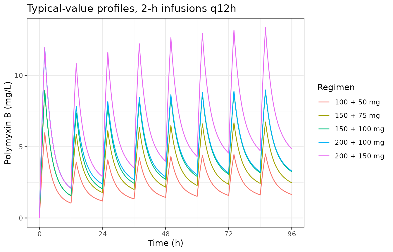
Visual predictive check
Figure 2 of the paper is a prediction-corrected VPC of the observed data around the seventh dose. Its dosing records are not published, so the check below simulates a representative regimen from Table 1 – a 100 mg loading dose (the median) followed by 75 mg q12h (the median daily dose of 150 mg), infused over 1 h – and plots the 5th, 50th and 95th percentiles over the seventh dosing interval (72-84 h), with residual error, against time after the start of the infusion. The paper’s figure shows a median near 4 mg/L at the end of the infusion falling to about 1.5 mg/L by the end of the interval.
vpc_ids <- seq_len(n_per_arm)
vpc_events <- dplyr::bind_rows(
  make_doses(vpc_ids, ld = 100, md = 75, dur = 1),
  make_obs(vpc_ids, seq(72, 96, by = 0.5))
) |>
  dplyr::arrange(id, time, dplyr::desc(evid)) |>
  as.data.frame()

vpc_sim <- rxode2::rxSolve(mod, vpc_events, returnType = "data.frame")
#> ℹ parameter labels from comments will be replaced by 'label()'
#> ℹ omega/sigma items treated as zero: 'etalq', 'etalvp'

vpc_q <- vpc_sim |>
  dplyr::mutate(tad = time - 72) |>
  dplyr::filter(tad <= 12) |>
  dplyr::group_by(tad) |>
  dplyr::summarise(
    p05 = quantile(sim, 0.05), p50 = quantile(sim, 0.50),
    p95 = quantile(sim, 0.95), .groups = "drop"
  )

ggplot2::ggplot(vpc_q, ggplot2::aes(tad)) +
  ggplot2::geom_ribbon(ggplot2::aes(ymin = p05, ymax = p95), alpha = 0.25) +
  ggplot2::geom_line(ggplot2::aes(y = p50)) +
  ggplot2::labs(x = "Time after start of the seventh dose (h)",
                y = "Polymyxin B (mg/L)",
                title = "Compare with Figure 2 of Tang 2023",
                subtitle = "100 mg load + 75 mg q12h, 1-h infusion; median and 90% interval") +
  ggplot2::theme_bw()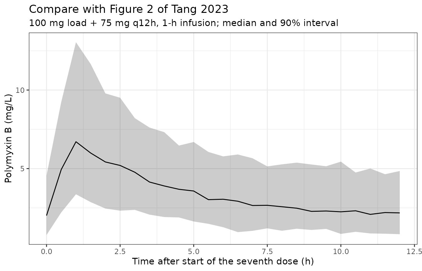
PKNCA validation
NCA is run on the individual predictions (Cc, no
residual error) of the same 200-subject cohort over day 4 (72-96 h), the
dosing day the paper uses for its steady-state exposure summaries. The
filter is !is.na(Cc) only, so the record at the start of
the interval is kept.
sim_nca <- vpc_sim |>
  dplyr::filter(!is.na(Cc)) |>
  dplyr::transmute(id, time = time - 72, Cc,
                   treatment = "100 mg + 75 mg q12h")

stopifnot(
  all(tapply(sim_nca$time, sim_nca$id, function(x) any(x == 0))),
  all(tapply(sim_nca$time, sim_nca$id, function(x) any(x == 24)))
)

conc_obj <- PKNCA::PKNCAconc(as.data.frame(sim_nca),
                             Cc ~ time | treatment + id,
                             concu = "mg/L", timeu = "h")
dose_df <- tidyr::expand_grid(id = vpc_ids, time = c(0, 12)) |>
  dplyr::mutate(amt = 75, treatment = "100 mg + 75 mg q12h") |>
  as.data.frame()
dose_obj <- PKNCA::PKNCAdose(dose_df, amt ~ time | treatment + id,
                             doseu = "mg")

intervals <- data.frame(start = 0, end = 24, cmax = TRUE, cmin = TRUE,
                        auclast = TRUE)
nca_res <- PKNCA::pk.nca(PKNCA::PKNCAdata(conc_obj, dose_obj,
                                          intervals = intervals))
The paper reports the cohort medians of the empirical-Bayes steady-state exposures (Results, “Population PK Model and polymyxin B exposure”): Cmin,ss 1.9 mg/L, Cmax,ss 5.9 mg/L and AUCss,24h 67.2 mg*h/L. Those were computed at each patient’s own regimen, not at one fixed regimen, so the comparison is a scale check rather than a replication.
published <- data.frame(
  treatment = "100 mg + 75 mg q12h",
  cmax = 5.9, cmin = 1.9, auclast = 67.2
)

cmp_nca <- nlmixr2lib::ncaComparisonTable(
  simulated = nca_res,
  reference = published,
  by = "treatment",
  units = c(cmax = "mg/L", cmin = "mg/L", auclast = "mg*h/L"),
  tolerance_pct = 20
)
knitr::kable(cmp_nca,
caption = "Simulated day-4 medians vs. the paper's EBE medians. * differs by >20%.")| NCA parameter | treatment | Reference | Simulated | % diff |
|---|---|---|---|---|
| Cmax (mg/L) | 100 mg + 75 mg q12h | 5.9 | 7.11 | +20.5%* |
| Cmin (mg/L) | 100 mg + 75 mg q12h | 1.9 | 2.12 | +11.5% |
| AUClast (mg*h/L) | 100 mg + 75 mg q12h | 67.2 | 87.1 | +29.6%* |
attr(cmp_nca, "footnote")
#> [1] "* differs from reference by more than ±20%."

nca_med <- as.data.frame(nca_res) |>
  dplyr::group_by(PPTESTCD) |>
  dplyr::summarise(med = median(PPORRES), .groups = "drop")
nca_med <- setNames(nca_med$med, nca_med$PPTESTCD)

# Typical-value day-4 AUC of the same regimen. AUC is monotone in the single
# shared eta, so the cohort median AUC estimates exactly this value; the
# sampling SE of a 200-subject median is about 3.5%.
tv_day4 <- rxode2::rxSolve(
  mod_tv,
  dplyr::bind_rows(make_doses(1L, ld = 100, md = 75, dur = 1),
                   make_obs(1L, seq(72, 96, by = 0.5))) |>
    dplyr::arrange(id, time, dplyr::desc(evid)) |>
    as.data.frame(),
  returnType = "data.frame"
) |>
  dplyr::filter(!is.na(Cc)) |>
  dplyr::transmute(id = 1L, time = time - 72, Cc)
#> ℹ omega/sigma items treated as zero: 'etalcl', 'etalq', 'etalvp'
tv_auc <- as.data.frame(PKNCA::pk.nca(PKNCA::PKNCAdata(
  PKNCA::PKNCAconc(tv_day4, Cc ~ time | id),
  intervals = data.frame(start = 0, end = 24, auclast = TRUE)
)))$PPORRES
#> No dose information provided, calculations requiring dose will return NA.

# Day 4 is close to steady state: the typical AUC sits just below the closed
# form 150 mg/day / 1.56 L/h = 96.2 mg*h/L. A mis-transcribed CL, volume or
# unit moves either check by tens of percent.
stopifnot(
  abs(tv_auc / (150 / 1.56) - 1) < 0.15,
  abs(nca_med[["auclast"]] / tv_auc - 1) < 0.12
)
The simulated Cmin agrees with the published median, but the simulated Cmax is about 20% higher and the AUC over 24 h about 30% higher. The gap is in the paper’s own numbers rather than in the model: at steady state AUCss,24h equals the daily dose divided by CL, and the paper’s subgroup medians (Table 3) of 144.7 mg/day with an AUC of 78.6 mgh/L in the clinical-success group and 117.0 mg/day with 60.6 mgh/L in the clinical-failure group both imply an apparent clearance of about 1.84-1.93 L/h, roughly 20% above the typical 1.56 L/h of Table 2. The paper’s own Monte Carlo simulation (Figure 6) is reproduced closely below with the Table 2 values, so the model is encoded as printed and the difference is left unexplained. The assumed 1-h infusion of this comparison regimen also raises the simulated Cmax relative to patients infused over longer times.
Replicate Figure 6: probability of target attainment
Figure 6 gives the probability of attaining AUC/MIC >= 66.9 (the
clinical cutoff from the paper’s ROC analysis) on day 1 (0-24 h) and day
4 (72-96 h) for each regimen. Because the model has a single random
effect – etalcl, shared by CL and Vc – each subject’s day-1
and day-4 AUC is a monotonically decreasing function of that one draw.
The PTA is therefore computed exactly, without Monte Carlo noise: solve
over a fine grid of etalcl, integrate AUC with PKNCA, find
the etalcl at which AUC equals 66.9 x MIC, and take the
normal probability below it.
omega_cl <- sqrt(rxode2::rxode(mod)$omega["etalcl", "etalcl"])
#> ℹ parameter labels from comments will be replaced by 'label()'
eta_grid <- seq(-1.6, 1.6, by = 0.05)

grid <- tidyr::expand_grid(regimens, etalcl = eta_grid) |>
  dplyr::mutate(id = dplyr::row_number())

pta_events <- dplyr::bind_rows(
  lapply(seq_len(nrow(regimens)), function(i) {
    ids <- grid$id[grid$regimen == regimens$regimen[i]]
    make_doses(ids, regimens$ld[i], regimens$md[i], dur = 2)
  }),
  make_obs(grid$id, c(seq(0, 24, by = 0.1), seq(72, 96, by = 0.1)))
) |>
  dplyr::arrange(id, time, dplyr::desc(evid)) |>
  as.data.frame()

pta_sim <- rxode2::rxSolve(
  mod_tv, pta_events,
  params = as.data.frame(grid[, c("id", "etalcl")]),
  returnType = "data.frame"
) |>
  dplyr::filter(!is.na(Cc)) |>
  dplyr::select(id, time, Cc)
#> ℹ omega/sigma items treated as zero: 'etalq', 'etalvp'
#> Warning: multi-subject simulation without without 'omega'

pta_conc <- PKNCA::PKNCAconc(pta_sim, Cc ~ time | id)
pta_res <- PKNCA::pk.nca(PKNCA::PKNCAdata(
  pta_conc,
  intervals = data.frame(start = c(0, 72), end = c(24, 96), auclast = TRUE)
))
#> No dose information provided, calculations requiring dose will return NA.

auc_grid <- as.data.frame(pta_res) |>
  dplyr::filter(PPTESTCD == "auclast") |>
  dplyr::mutate(day = ifelse(start == 0, "Day 1", "Day 4")) |>
  dplyr::select(id, day, auc = PPORRES) |>
  dplyr::left_join(grid, by = "id")

# Monotone in the shared eta, so a single crossing defines the PTA.
stopifnot(all(
  auc_grid |>
    dplyr::group_by(regimen, day) |>
    dplyr::arrange(etalcl, .by_group = TRUE) |>
    dplyr::summarise(mono = all(diff(auc) < 0), .groups = "drop") |>
    dplyr::pull(mono)
))
pta_one <- function(eta, auc, target) {
  f <- stats::approxfun(eta, auc - target)
  if (f(max(eta)) >= 0) return(1)
  if (f(min(eta)) <= 0) return(0)
  stats::pnorm(stats::uniroot(f, range(eta))$root / omega_cl)
}

mics <- c(0.125, 0.25, 0.5, 1, 2, 4, 8)
pta <- auc_grid |>
  tidyr::expand_grid(mic = mics) |>
  dplyr::group_by(regimen, day, mic) |>
  dplyr::summarise(pta = 100 * pta_one(etalcl, auc, 66.9 * mic[1]),
                   .groups = "drop")

ggplot2::ggplot(pta, ggplot2::aes(mic, pta, colour = regimen)) +
  ggplot2::geom_line() +
  ggplot2::geom_point() +
  ggplot2::geom_hline(yintercept = 90, linetype = "dashed") +
  ggplot2::scale_x_continuous(trans = "log2", breaks = mics) +
  ggplot2::facet_wrap(~day, ncol = 1) +
  ggplot2::labs(x = "MIC (mg/L)", y = "PTA (%)", colour = "Loading + q12h",
                title = "Replicates Figure 6 of Tang 2023",
                subtitle = "Target AUC/MIC >= 66.9; dashed line is 90%") +
  ggplot2::theme_bw()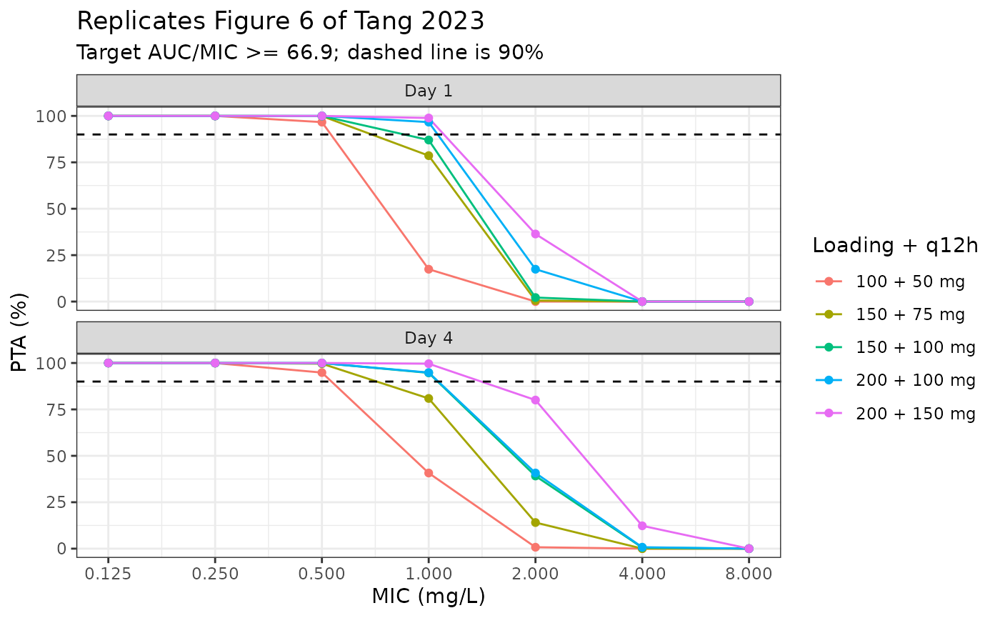
The table compares the exact PTA with values read by eye from Figure 6 at the MICs where the curves are not at 0% or 100%.
fig6 <- tibble::tribble(
  ~regimen,        ~day,    ~mic, ~fig,
  "100 + 50 mg",   "Day 1",  0.5,   96,
  "100 + 50 mg",   "Day 1",  1,     16,
  "150 + 75 mg",   "Day 1",  1,     78,
  "150 + 100 mg",  "Day 1",  1,     86,
  "200 + 100 mg",  "Day 1",  1,     96,
  "200 + 100 mg",  "Day 1",  2,     16,
  "200 + 150 mg",  "Day 1",  2,     35,
  "100 + 50 mg",   "Day 4",  0.5,   95,
  "100 + 50 mg",   "Day 4",  1,     42,
  "150 + 75 mg",   "Day 4",  1,     81,
  "150 + 75 mg",   "Day 4",  2,     15,
  "150 + 100 mg",  "Day 4",  1,     94,
  "150 + 100 mg",  "Day 4",  2,     40,
  "200 + 100 mg",  "Day 4",  1,     95,
  "200 + 100 mg",  "Day 4",  2,     42,
  "200 + 150 mg",  "Day 4",  2,     81,
  "200 + 150 mg",  "Day 4",  4,     13
) |>
  dplyr::mutate(regimen = factor(regimen, levels = levels(regimens$regimen)))

pta_cmp <- fig6 |>
  dplyr::left_join(pta, by = c("regimen", "day", "mic")) |>
  dplyr::mutate(pta = round(pta, 1), diff = round(pta - fig, 1))

pta_cmp |>
  dplyr::rename("Regimen" = regimen, "Day" = day, "MIC (mg/L)" = mic,
                "Figure 6 PTA (%)" = fig, "Model PTA (%)" = pta,
                "Difference (points)" = diff) |>
knitr::kable(caption = "Exact model PTA vs. Figure 6 of Tang 2023 (read by eye).")| Regimen | Day | MIC (mg/L) | Figure 6 PTA (%) | Model PTA (%) | Difference (points) |
|---|---|---|---|---|---|
| 100 + 50 mg | Day 1 | 0.5 | 96 | 96.7 | 0.7 |
| 100 + 50 mg | Day 1 | 1.0 | 16 | 17.4 | 1.4 |
| 150 + 75 mg | Day 1 | 1.0 | 78 | 78.6 | 0.6 |
| 150 + 100 mg | Day 1 | 1.0 | 86 | 87.0 | 1.0 |
| 200 + 100 mg | Day 1 | 1.0 | 96 | 96.7 | 0.7 |
| 200 + 100 mg | Day 1 | 2.0 | 16 | 17.4 | 1.4 |
| 200 + 150 mg | Day 1 | 2.0 | 35 | 36.4 | 1.4 |
| 100 + 50 mg | Day 4 | 0.5 | 95 | 94.8 | -0.2 |
| 100 + 50 mg | Day 4 | 1.0 | 42 | 40.7 | -1.3 |
| 150 + 75 mg | Day 4 | 1.0 | 81 | 80.9 | -0.1 |
| 150 + 75 mg | Day 4 | 2.0 | 15 | 14.1 | -0.9 |
| 150 + 100 mg | Day 4 | 1.0 | 94 | 94.7 | 0.7 |
| 150 + 100 mg | Day 4 | 2.0 | 40 | 39.1 | -0.9 |
| 200 + 100 mg | Day 4 | 1.0 | 95 | 94.8 | -0.2 |
| 200 + 100 mg | Day 4 | 2.0 | 42 | 40.7 | -1.3 |
| 200 + 150 mg | Day 4 | 2.0 | 81 | 80.0 | -1.0 |
| 200 + 150 mg | Day 4 | 4.0 | 13 | 12.3 | -0.7 |
# Deterministic (no random draws); the residual is reading error on the figure.
stopifnot(max(abs(pta_cmp$diff)) < 6)
The exact PTA matches every legible point of Figure 6 within the precision of reading the figure, which confirms the structural values, the size of the CL variability and the shared CL-Vc random effect as encoded. In particular it reproduces the paper’s conclusions: 75 mg q12h reaches >= 90% PTA at MIC <= 0.5 mg/L, 100 mg q12h reaches it at MIC 1 mg/L by day 4, no regimen reaches it at the 2 mg/L breakpoint, and a loading dose is needed for day-1 attainment.
Assumptions and deviations
The 100% CL-Vc correlation is a shared random effect. Table 2 reports the CL-Vc correlation as 100. A 2 x 2 omega block with correlation 1 is singular and cannot be sampled, so Vc reuses the CL random effect scaled by
vc_eta_scale = omega_Vc / omega_CL = 0.286 / 0.394. This gives the published SD for each and a correlation of exactly 1. The scaling factor is derived from the two printed omegas, not estimated by the authors.The omega percentages are read on the SD scale. Table 2 reports “omega CL” = 39.4% and “omega Vc” = 28.6% under “Random effect (%)” without defining the percentage. They are read as
omega = pct / 100, as in the sibling polymyxin B models. Reading them instead as log-normal CVs (omega^2 = log(1 + CV^2)) gives 0.381 and 0.281, which changes the Figure 6 PTA by under 2 percentage points; the figure cannot discriminate between the two.IIV on CLd and Vp is zero. The authors held both variances at 0 because their shrinkage exceeded 50%; they are kept as zero-variance random effects.
Day definitions for Figure 6. The paper does not define “day 1” and “day 4”; they are taken as 0-24 h and 72-96 h from the first (loading) dose, with doses every 12 h and 2-h infusions as stated in the Methods.
EBE exposure medians are not reproduced. The paper’s empirical-Bayes AUCss,24h medians imply an apparent clearance about 20% above the typical value of Table 2 (see the PKNCA section). Figure 6, which the paper computed from the same model, is reproduced closely, so the published estimates are used unchanged.
The efficacy model is not encoded. The multivariable logistic regression of clinical efficacy on AUCss,24h/MIC, daily dose and inhaled polymyxin B (Table 3) is reported only as adjusted odds ratios, without an intercept, so it cannot be turned into a predictive model. The AUC/MIC cutoff of 66.9 from the paper’s ROC analysis is used as the Figure 6 target above.
Inhaled polymyxin B is not modelled. 34 patients also received nebulized polymyxin B; the PK model describes the intravenous dose only.