Lamivudine (Bouazza 2010)
Source:vignettes/articles/Bouazza_2010_lamivudine.Rmd
Bouazza_2010_lamivudine.RmdModel and source
mod <- rxode2::rxode2(readModelDb("Bouazza_2010_lamivudine"))
#> ℹ parameter labels from comments will be replaced by 'label()'- Citation: Bouazza N et al. Is the recommended once-daily dose of lamivudine optimal in West African HIV-infected children? Antimicrob Agents Chemother. 2010;54(9):3938-3943. doi:10.1128/AAC.00306-10
- Article: https://doi.org/10.1128/AAC.00306-10
- Trial: BURKINAME-ANRS 12103 (ClinicalTrials.gov NCT00122538)
Population
The fit population was 45 antiretroviral-naive HIV-1 infected children (17 girls, 28 boys; age 2.5-14 years, median 6.75 years; body weight 11-37 kg, median 16.8 kg) enrolled in the BURKINAME-ANRS 12103 trial in Bobo-Dioulasso, Burkina Faso. All received once-daily oral lamivudine 8 mg/kg (median 150 mg, range 90-300 mg) as 150 mg tablet or 10 mg/mL solution, co-administered with didanosine 240 mg/m^2 and weight-band efavirenz. A total of 148 plasma lamivudine concentrations were analysed. Baseline demographics and laboratory covariates (serum creatinine, ALAT, ASAT, total bilirubin) are summarised in Table 1 of the source.
The same fields are available programmatically:
mod$population
#> $species
#> [1] "human"
#>
#> $n_subjects
#> [1] 45
#>
#> $n_studies
#> [1] 1
#>
#> $age_range
#> [1] "2.5-14 years (median 6.75)"
#>
#> $age_median
#> [1] "6.75 years"
#>
#> $weight_range
#> [1] "11-37 kg"
#>
#> $weight_median
#> [1] "16.8 kg"
#>
#> $sex_female_pct
#> [1] 38
#>
#> $race_ethnicity
#> [1] "West African (sub-Saharan); ethnic stratification not reported in source."
#>
#> $disease_state
#> [1] "Antiretroviral-naive HIV-1 infected children, CDC clinical stage A-C, with severe immunological / virological status meeting Burkina Faso HAART initiation criteria."
#>
#> $dose_range
#> [1] "Lamivudine oral, 8 mg/kg once daily as 150 mg tablet or 10 mg/ml oral solution; median dose 150 mg (range 90-300 mg). Co-administered with didanosine 240 mg/m^2 q.d. and weight-band efavirenz q.d."
#>
#> $regions
#> [1] "Burkina Faso (Bobo-Dioulasso); BURKINAME-ANRS 12103 trial (ClinicalTrials.gov NCT00122538)."
#>
#> $n_observations
#> [1] 148
#>
#> $notes
#> [1] "Forty-nine children enrolled, 45 evaluable for PK (17 girls / 28 boys). Sampling schedule: pre-dose, 1 h, 3 h post-dose (39 children) or pre-dose, 1, 2, 3, 6, 12, 24 h post-dose (10 children). Sampling began on day 15 of treatment for 38 children and between months 2-5 of treatment for 11 children -- assumed to be at steady state for the model. Demographics in Table 1 of the source."
Structural model
The final model is a two-compartment model with first-order absorption. Sampling in this trial did not capture the absorption phase, so Ka was set equal to the distribution-phase eigenvalue (alpha) of the disposition model. Ka was further fixed at 0.71 1/h, the value reported in an earlier paediatric lamivudine PK study (Tremoulet et al., reference 17 of the source). With the final point estimates this constraint is internally consistent: the disposition eigenvalues computed from CL/F, Vc/F, Q/F, Vp/F at the cohort median weight are alpha = 0.71 and beta = 0.059 1/h, so absorption and distribution rates coincide as assumed.
After allometric scaling of CL/F, Q/F (exponent 0.75) and Vc/F, Vp/F (exponent 1) to the cohort-median body weight of 16.8 kg, no further covariate (age, serum creatinine, amylase, ALAT, ASAT, total bilirubin, or formulation) reached the OFV cut-off of 6.63 units. Inter-subject variability was retained only on CL/F and described by an exponential model; residual variability was a multiplicative (proportional) error.
Source trace
| Element | Value | Source location |
|---|---|---|
| Two-compartment ODE structure | n/a | Results “Population pharmacokinetics” paragraph 1 |
| Ka = alpha constraint | n/a | Methods “Modeling strategy” |
| Allometric exponents | 0.75, 1 | Methods “Modeling strategy” (theoretical values) |
| Reference body weight | 16.8 kg | Table 2 footer (“standardized for a median weight of 16.8 kg”) |
| Ka | 0.71 1/h | Table 2 (fixed; reference 17) |
| CL/F | 16.9 L/h | Table 2 |
| Vc/F | 30.8 L | Table 2 |
| Vp/F | 58.6 L | Table 2 |
| Q/F | 4.48 L/h | Table 2 |
| omega(CL/F) | 0.30 | Table 2 (interpreted as SD on log scale; see Assumptions) |
| sigma (proportional SD) | 0.60 | Table 2 (multiplicative error model) |
Virtual cohort
set.seed(20100601)

n_sim <- 1000
# Body-weight distribution matched to Table 1 of the source:
# range 11-37 kg, median 16.8 kg. Use a truncated log-normal anchored on the
# median to approximate the right-skewed paediatric distribution without
# overstating tail weights.
wts <- rlnorm(n_sim, meanlog = log(16.8), sdlog = 0.30)
wts <- pmin(pmax(wts, 11), 37)

# Three weight strata for the dose-recommendation analyses:
#   "<17 kg"  - cohort median is 14 kg; recommended dose 10 mg/kg per source.
#   ">=17 kg" - recommended dose 8 mg/kg per source.
# The source's tree-regression cut-off was 17 kg.
make_cohort <- function(WTs, dose_mgkg, regimen_label, id_offset = 0L) {
  n <- length(WTs)
  ids <- id_offset + seq_len(n)
  obs_times <- seq(0, 24*7, by = 0.5)

  doses <- data.frame(
    id   = ids,
    time = 0,
    amt  = dose_mgkg * WTs,
    cmt  = "depot",
    evid = 1L
  )
  # Dose every 24 h for one week (steady state)
  dose_rows <- do.call(rbind, lapply(0:6, function(d) {
    out <- doses
    out$time <- d * 24
    out
  }))

  obs <- expand.grid(id = ids, time = obs_times)
  obs$amt <- 0
  obs$cmt <- NA
  obs$evid <- 0L

  evt <- dplyr::bind_rows(dose_rows, obs)
  evt$WT <- WTs[match(evt$id - id_offset, seq_len(n))]
  evt$regimen <- regimen_label
  evt[order(evt$id, evt$time, -evt$evid), ]
}

events <- dplyr::bind_rows(
  make_cohort(wts[wts <  17], dose_mgkg =  8, regimen_label = "<17 kg, 8 mg/kg q.d.",  id_offset =      0L),
  make_cohort(wts[wts <  17], dose_mgkg = 10, regimen_label = "<17 kg, 10 mg/kg q.d.", id_offset =  20000L),
  make_cohort(wts[wts >= 17], dose_mgkg =  8, regimen_label = ">=17 kg, 8 mg/kg q.d.", id_offset =  40000L)
)
stopifnot(!anyDuplicated(unique(events[, c("id", "time", "evid")])))
Simulation
sim <- rxode2::rxSolve(mod, events = events, keep = c("regimen", "WT"))
sim <- as.data.frame(sim)
Replicate published NCA – Table 3 (“This study” row)
Bouazza 2010 Table 3 reports per-cohort NCA values (geometric mean per the narrative, although the row label is “Median (95% CI)” with IQR-like spreads): Cmin = 0.04 mg/L (range 0.01-0.14), Cmax = 1.7 mg/L (range 1.34-2.01), AUC0-tau = 7.8 mg*h/L (range 4.72-14.27), CL/F = 1.03 L/h/kg (range 0.55-1.62). These were computed at the actually-administered dose of 8 mg/kg q.d., pooling all 45 children regardless of body weight.
The block below reproduces the same NCA pooling all simulated subjects on the 8 mg/kg q.d. regimen (the < 17 kg and >= 17 kg sub-cohorts combined) so the comparison is dose- and regimen-matched.
last_dose <- 6 * 24
sim_ss <- sim |>
  dplyr::filter(time >= last_dose, time <= last_dose + 24,
                regimen %in% c("<17 kg, 8 mg/kg q.d.", ">=17 kg, 8 mg/kg q.d.")) |>
  dplyr::mutate(time = time - last_dose,
                regimen = "8 mg/kg q.d. (pooled)") |>
  dplyr::select(id, time, Cc, regimen, WT)

dose_df <- events |>
  dplyr::filter(evid == 1, time == last_dose,
                regimen %in% c("<17 kg, 8 mg/kg q.d.", ">=17 kg, 8 mg/kg q.d.")) |>
  dplyr::mutate(time = 0,
                regimen = "8 mg/kg q.d. (pooled)") |>
  dplyr::select(id, time, amt, regimen, WT)

conc_obj <- PKNCA::PKNCAconc(sim_ss, Cc ~ time | regimen + id)
dose_obj <- PKNCA::PKNCAdose(dose_df, amt ~ time | regimen + id)

intervals <- data.frame(
  start    = 0,
  end      = 24,
  cmax     = TRUE,
  tmax     = TRUE,
  cmin     = TRUE,
  auclast  = TRUE,
  cl.last  = TRUE
)

nca_res <- PKNCA::pk.nca(PKNCA::PKNCAdata(conc_obj, dose_obj, intervals = intervals))
nca_tbl <- as.data.frame(nca_res$result)

simulated_summary <- nca_tbl |>
  dplyr::filter(PPTESTCD %in% c("cmax", "cmin", "auclast", "cl.last")) |>
  dplyr::group_by(PPTESTCD) |>
  dplyr::summarise(
    median = stats::median(PPORRES, na.rm = TRUE),
    p05    = stats::quantile(PPORRES, 0.05, na.rm = TRUE),
    p95    = stats::quantile(PPORRES, 0.95, na.rm = TRUE),
    .groups = "drop"
  )

# CL/F per kg: PKNCA cl.last has units 1/h after dividing by AUC of
# dose-normalised concentration; convert to L/h/kg by dose / AUC / WT.
clf_per_kg <- nca_tbl |>
  dplyr::filter(PPTESTCD == "auclast") |>
  dplyr::left_join(
    dose_df |> dplyr::select(id, amt, WT) |> dplyr::distinct(),
    by = "id"
  ) |>
  dplyr::mutate(clf_kg = amt / PPORRES / WT) |>
  dplyr::summarise(
    median = stats::median(clf_kg, na.rm = TRUE),
    p05    = stats::quantile(clf_kg, 0.05, na.rm = TRUE),
    p95    = stats::quantile(clf_kg, 0.95, na.rm = TRUE)
  ) |>
  dplyr::mutate(PPTESTCD = "clf_kg") |>
  dplyr::select(PPTESTCD, dplyr::everything())

simulated_summary <- dplyr::bind_rows(simulated_summary, clf_per_kg)

published <- tibble::tibble(
  PPTESTCD = c("cmin",  "cmax",  "auclast", "clf_kg"),
  pub_value = c(0.04,    1.7,     7.8,       1.03),
  pub_range = c("0.01-0.14", "1.34-2.01", "4.72-14.27", "0.55-1.62")
)

comparison <- published |>
  dplyr::left_join(simulated_summary, by = "PPTESTCD") |>
  dplyr::transmute(
    Parameter      = PPTESTCD,
    `Published`    = paste0(pub_value, " (", pub_range, ")"),
    `Simulated`    = sprintf("%.3f (%.3f-%.3f)", median, p05, p95)
  )

knitr::kable(comparison,
caption = "Simulated steady-state lamivudine NCA at 8 mg/kg q.d., pooled across the cohort body-weight range, vs Table 3 'This study' values.")| Parameter | Published | Simulated |
|---|---|---|
| cmin | 0.04 (0.01-0.14) | 0.041 (0.015-0.114) |
| cmax | 1.7 (1.34-2.01) | 1.672 (1.318-2.053) |
| auclast | 7.8 (4.72-14.27) | 7.910 (4.814-13.138) |
| clf_kg | 1.03 (0.55-1.62) | 1.011 (0.609-1.662) |
Replicate Figure 3 – CL/F (L/h/kg) vs body weight
Figure 3 of the source plots apparent elimination clearance in L/h/kg
against body weight, with the line representing the allometric model
CL/F per kg = CL_pop/WT_pop * (WT/WT_pop)^(0.75 - 1). The
block below reproduces the same curve using the typical-value model
(zeroRe()) over the cohort weight range.
wt_grid <- seq(10, 40, length.out = 200)
allom_clf_per_kg <- 16.9 / 16.8 * (wt_grid / 16.8)^(0.75 - 1)

ggplot(data.frame(WT = wt_grid, CLF_per_kg = allom_clf_per_kg),
       aes(WT, CLF_per_kg)) +
  geom_line(linewidth = 1) +
  geom_vline(xintercept = 17, linetype = 3) +
  labs(x = "Body weight (kg)",
       y = "Apparent CL/F (L/h/kg)",
       title = "Figure 3 -- allometric CL/F (per kg) vs body weight",
       caption = "Replicates the model curve in Figure 3 of Bouazza 2010. Dotted line: tree-regression cut-off (17 kg).")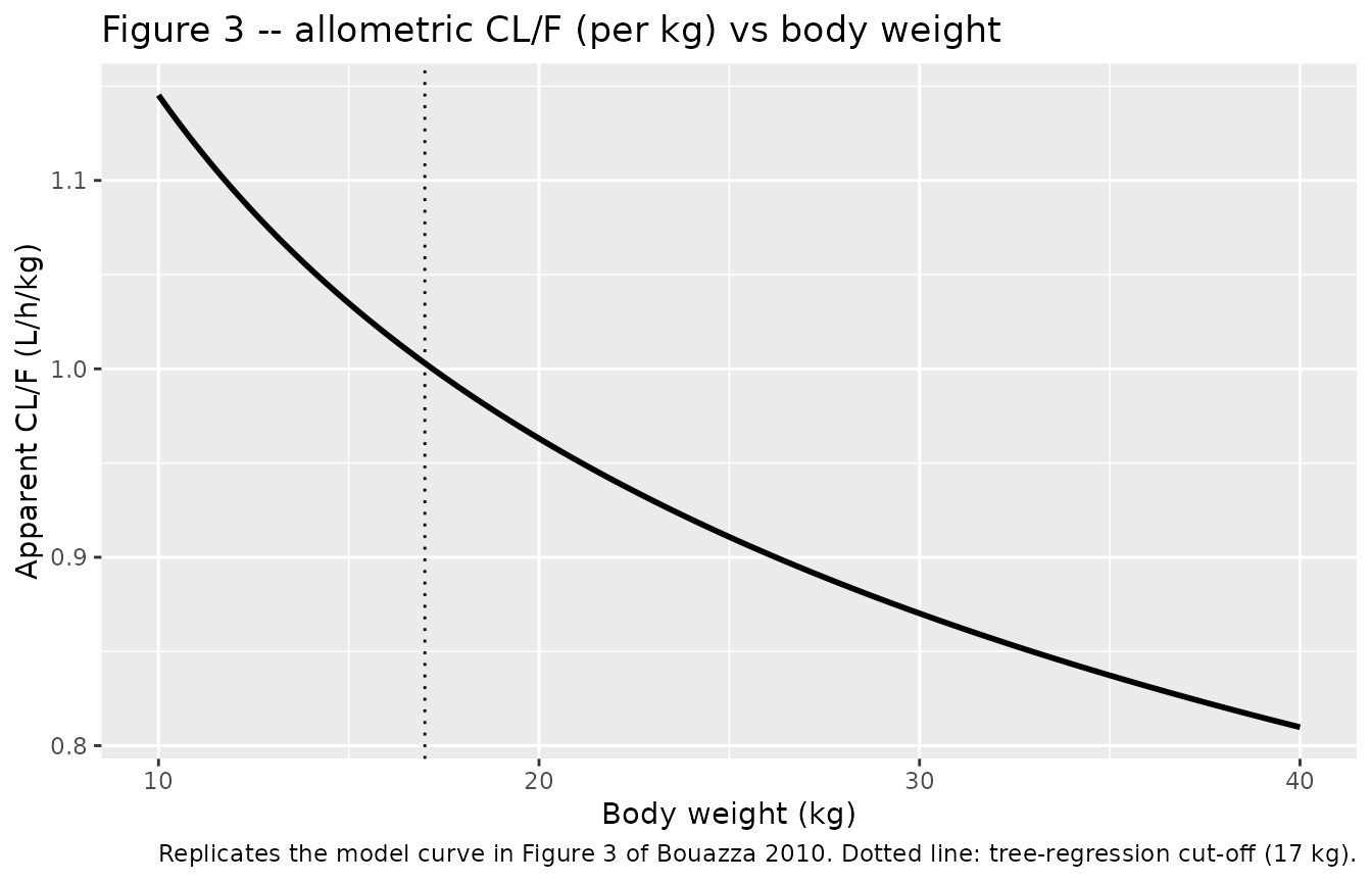
Replicate Figure 4 – mean AUC by dose, by weight band
Figure 4 of the source displays the mean lamivudine AUC0-24 obtained by simulating 45,000 children (1,000 replicates of the database) at 8, 10, and 12 mg/kg q.d., split into the two body-weight bands defined by the tree-regression analysis. The horizontal line at AUC = 8.9 mg*h/L is the adult target.
# Add 12 mg/kg arms for both weight bands so the figure spans the published doses.
events_fig4 <- dplyr::bind_rows(
  events,
  make_cohort(wts[wts <  17], dose_mgkg = 12, regimen_label = "<17 kg, 12 mg/kg q.d.", id_offset =  60000L),
  make_cohort(wts[wts >= 17], dose_mgkg = 10, regimen_label = ">=17 kg, 10 mg/kg q.d.", id_offset =  80000L),
  make_cohort(wts[wts >= 17], dose_mgkg = 12, regimen_label = ">=17 kg, 12 mg/kg q.d.", id_offset = 100000L)
)
stopifnot(!anyDuplicated(unique(events_fig4[, c("id", "time", "evid")])))

sim_fig4 <- as.data.frame(
  rxode2::rxSolve(mod, events = events_fig4, keep = c("regimen", "WT"))
)

auc_summary <- sim_fig4 |>
  dplyr::filter(time >= last_dose, time <= last_dose + 24) |>
  dplyr::mutate(time = time - last_dose) |>
  dplyr::group_by(regimen, id) |>
  dplyr::summarise(
    AUC024 = sum(diff(time) * (utils::head(Cc, -1) + utils::tail(Cc, -1)) / 2),
    .groups = "drop"
  ) |>
  tidyr::separate(regimen, into = c("band", "dose"), sep = ", ", remove = FALSE) |>
  dplyr::mutate(dose_mgkg = as.numeric(sub(" mg/kg q.d.", "", dose)))

auc_band <- auc_summary |>
  dplyr::group_by(band, dose_mgkg) |>
  dplyr::summarise(
    AUC_mean = mean(AUC024),
    AUC_lo   = stats::quantile(AUC024, 0.025),
    AUC_hi   = stats::quantile(AUC024, 0.975),
    .groups  = "drop"
  )

ggplot(auc_band, aes(dose_mgkg, AUC_mean, colour = band, group = band)) +
  geom_point(size = 2) +
  geom_line() +
  geom_errorbar(aes(ymin = AUC_lo, ymax = AUC_hi), width = 0.3) +
  geom_hline(yintercept = 8.9, linetype = 1) +
  geom_hline(yintercept = c(5.2, 12.6), linetype = 2) +
  labs(x = "Lamivudine dose (mg/kg q.d.)",
       y = "Mean steady-state AUC0-24 (mg*h/L)",
       colour = "Body-weight band",
       title = "Figure 4 -- mean AUC0-24 by dose and body-weight band",
       caption = paste("Replicates Figure 4 of Bouazza 2010. Solid line: adult target 8.9 mg*h/L.",
                       "Dashed lines: adult 95% CI 5.2-12.6 mg*h/L.")) +
  theme(legend.position = "bottom")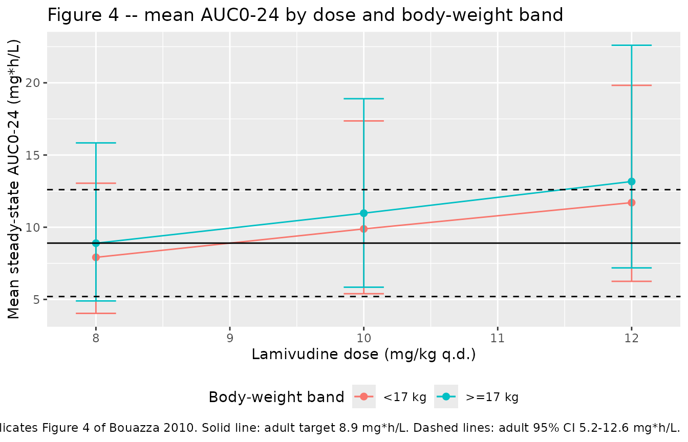
Assumptions and deviations
-
Omega and sigma scale. Bouazza 2010 Table 2 reports
the random-effect point estimates as
omega(CL/F) = 0.30andsigma = 0.60without explicit annotation of whether they are SDs or variances. The same author group’s follow-up Bouazza 2011 Antimicrob Agents Chemother paper (PMID 21576437) on lamivudine in 580 children reportsomega CL/F = 0.32in Table 1, paired with(32%)in the abstract – i.e. the omega is the SD on the log scale (approximately CV when small). This vignette adopts the same convention for the 2010 fit:omega(CL/F) = 0.30is encoded as variance0.30^2 = 0.09on the nlmixr2etalclline, andsigma = 0.60is encoded as the proportional SDpropSd <- 0.60. The published Cmax, Cmin, and AUC ranges in Table 3 are reproduced under this reading (see the NCA comparison above). -
Ka structurally fixed. Ka was fixed to 0.71 1/h per
the source, taken from a prior paediatric lamivudine study (Tremoulet et
al., reference 17 of the source). The literature value also coincides
with the alpha disposition eigenvalue implied by the fitted CL/F, Q/F,
Vc/F, Vp/F, so the “Ka = alpha” structural constraint is
self-consistent. The packaged model encodes Ka as
fixed(log(0.71)). - Body-weight distribution. The original individual covariates are not publicly available. The virtual cohort uses a log-normal weight distribution anchored on the cohort median (16.8 kg) and clipped to the source range (11-37 kg). The < 17 kg and >= 17 kg strata reproduce the tree-regression groups described in Results.
- Steady-state simulation. The source PK study was conducted between day 15 and month 5 of treatment; observations were treated as steady state in the model fit. The vignette reproduces this by simulating six daily doses before the analysis interval.
- Galenic form not encoded. Bouazza 2010 tested an oral-tablet vs oral-solution effect on bioavailability and found no significant difference; the packaged model therefore does not carry a formulation covariate.
- No covariate beyond body weight. After allometric scaling, age and the biological covariates (serum creatinine, amylase, ALAT, ASAT, total bilirubin) did not improve the model. They are not part of the packaged model.