Naloxone (Dowling 2008)
Source:vignettes/articles/Dowling_2008_naloxone.Rmd
Dowling_2008_naloxone.RmdModel and source
- Citation: Dowling J, Isbister GK, Kirkpatrick CMJ, Naidoo D, Graudins A. Population pharmacokinetics of intravenous, intramuscular, and intranasal naloxone in human volunteers. Ther Drug Monit. 2008;30(4):490-496. doi:10.1097/FTD.0b013e3181816214
- Description: Three-compartment population PK model for naloxone in six healthy male volunteers receiving 0.8 mg intravenous, 0.8 mg intramuscular, 0.8 mg intranasal, 2 mg intravenous, and 2 mg intranasal doses in an open-label crossover design (Dowling 2008). Intramuscular and intranasal absorption are modeled as first-order via separate depot compartments (Ka_im 0.65 1/h, F_im 0.36; Ka_in 1.52 1/h, F_in 0.038); intravenous doses go directly to the central compartment (F 1, structural anchor). Fat-free mass (Janmahasatian 2005 formula, called LBW2005 in the paper) is allometrically scaled on clearance with fixed exponent 0.75, and body weight is linearly scaled on central volume (exponent 1); both effects use a 70 kg reference.
- Article: https://doi.org/10.1097/FTD.0b013e3181816214
Population
Six healthy adult male volunteers were enrolled in an open-label
single-site crossover study at Prince of Wales Hospital (Sydney,
Australia). Median age was 25 years (range 24-45), median weight 80 kg
(range 75-100), and median height 1.78 m (range 1.75-1.93). Exclusion
criteria were previous or current opioid dependence or abuse, current
use of opioid analgesics, cardiorespiratory disease, current or recent
upper respiratory tract infection, and abnormal nasal anatomy. Each
volunteer received naloxone on five occasions in the same order – 0.8 mg
IV, 0.8 mg IM, 0.8 mg IN, 2 mg IV, 2 mg IN – with a minimum 2-day
washout between doses. Blood samples were collected at 5, 10, 15, 30,
45, 60, 90, 120, 180, and 240 minutes post-dose. Because naloxone was
only detectable above the 1 ug/L LOQ in two subjects after 2 mg IN and
in no subjects after 0.8 mg IN, the final dataset contained 128
concentrations across four analyzable occasions (0.8 mg IV, 2 mg IV, 0.8
mg IM, and 2 mg IN) in six subjects. Race / ethnicity was not reported.
See Dowling 2008 Methods ‘Patient Data’ for the full baseline
description; the same fields are available programmatically via
readModelDb("Dowling_2008_naloxone")()$population.
Source trace
The per-parameter origin is recorded as an in-file comment next to
each ini() entry in
inst/modeldb/specificDrugs/Dowling_2008_naloxone.R. The
table below collects them in one place.
| Equation / parameter | Final value | Source location |
|---|---|---|
lka (Ka intramuscular) |
0.65 1/h | Table 1 |
lka2 (Ka intranasal) |
1.52 1/h | Table 1 |
lcl (Clearance) |
91 L/h | Table 1 |
lvc (Central volume V2) |
2.87 L | Table 1 |
lvp (First peripheral volume V3) |
1.49 L | Table 1 |
lvp2 (Second peripheral volume V4) |
33.6 L | Table 1 |
lq (Q3) |
5.66 L/h | Table 1 |
lq2 (Q4) |
29.8 L/h | Table 1 |
lfdepot (F intramuscular) |
0.36 | Table 1 |
lfdepot2 (F intranasal) |
0.038 | Table 1 |
e_ffm_cl (FFM allometric exponent on CL) |
0.75 (FIXED) | Results Section, printed CL equation |
e_wt_vc (WT linear exponent on V2) |
1 (FIXED) | Results Section, printed V2 equation |
etalcl (BSV on CL, omega^2) |
0.00581 (CV ~ 7.6%) | Table 1 |
etalvc (BSV on V2, omega^2) |
0.25 (CV ~ 50%) | Table 1 |
propSd (Proportional residual) |
sqrt(0.101) = 0.318 | Table 1 (Prop Err 0.101 (31.7%)) |
addSd (Additive residual, ng/mL) |
sqrt(0.001) = 0.0316 (FIXED) | Table 1 (Add Err 0.001 fixed) |
| Equation: 3-compartment disposition (central + peripheral1 + peripheral2) | n/a | Methods ‘Data Analysis’ and Table 1 |
| Equation: parallel first-order absorption via two depots (IM, IN); IV bolus to central | n/a | Methods ‘Data Analysis’ |
Equation:
CL = TVCL * (LBW2005/70)^0.75 * exp(etalcl)
|
n/a | Results Section, printed equation |
Equation: V2 = TVV2 * (WT/70) * exp(etalvc)
|
n/a | Results Section, printed equation |
Concentration units: model returns
Cc = 1000 * central / vc (mg/L -> ng/mL == ug/L) |
n/a | Methods ‘Patient Data’ (LOQ 1 ug/L) |
Virtual cohort
Individual patient concentrations from Dowling 2008 are not publicly
available. The simulations below use the Dowling 2008 Methods
‘Simulations’ setup: a uniform 70 kg male cohort simulated across the
four analyzable trial arms (0.8 mg IV, 2 mg IV, 0.8 mg IM, 2 mg IN).
Fat-free mass is computed via the Janmahasatian formula at a 70 kg /
1.78 m male reference: BMI = 22.09 kg/m^2 and FFM = 9.27e3 * 70 /
(6.68e3 + 216 * 22.09) = 56.55 kg. The trial-arm label rides through
rxSolve via keep = "treatment" so PKNCA can
stratify its output by dose group.
Cohort size: 200 subjects per arm (per the standing 200/arm cap for validation vignettes). The paper simulated 1000 per arm; 200 is ample for the median / 5th-95th VPC bands and keeps the render fast.
set.seed(20080730)

n_per_arm <- 200L

arms <- tibble::tribble(
  ~treatment,    ~dose_mg, ~cmt,
  "0.8 mg IV",    0.8,     "central",
  "2 mg IV",      2.0,     "central",
  "0.8 mg IM",    0.8,     "depot",
  "2 mg IN",      2.0,     "depot2"
)

obs_times <- c(seq(0, 0.5, by = 0.02), seq(0.6, 4, by = 0.1))

# Uniform 70 kg male, 1.78 m -> FFM via Janmahasatian
ref_wt_kg <- 70
ref_ht_m  <- 1.78
ref_bmi   <- ref_wt_kg / ref_ht_m^2
ref_ffm   <- 9.27e3 * ref_wt_kg / (6.68e3 + 216 * ref_bmi)

make_events_for_arm <- function(arm_row, n, id_offset) {
  ids <- id_offset + seq_len(n)
  dose_rows <- tibble::tibble(
    id        = ids,
    time      = 0,
    amt       = arm_row$dose_mg,
    evid      = 1L,
    cmt       = arm_row$cmt,
    treatment = arm_row$treatment,
    WT        = ref_wt_kg,
    FFM       = ref_ffm
  )
  obs_rows <- tidyr::expand_grid(id = ids, time = obs_times) |>
    dplyr::mutate(
      amt       = NA_real_,
      evid      = 0L,
      cmt       = "central",
      treatment = arm_row$treatment,
      WT        = ref_wt_kg,
      FFM       = ref_ffm
    )
  dplyr::bind_rows(dose_rows, obs_rows) |>
    dplyr::arrange(id, time, evid)
}

events <- dplyr::bind_rows(lapply(seq_len(nrow(arms)), function(i) {
  make_events_for_arm(arms[i, ], n_per_arm, id_offset = (i - 1L) * n_per_arm)
}))

stopifnot(!anyDuplicated(unique(events[, c("id", "time", "evid")])))
Simulation
mod <- readModelDb("Dowling_2008_naloxone")
sim <- rxode2::rxSolve(mod, events = events, keep = c("treatment")) |>
  as.data.frame() |>
  dplyr::mutate(treatment = factor(treatment, levels = arms$treatment))
#> ℹ parameter labels from comments will be replaced by 'label()'
Replicate published figures
Figure 2: visual predictive plots by arm
Dowling 2008 Figure 2 shows the 5th / 50th / 95th simulated concentration percentiles by time for each of the four analyzable arms. The panel below reproduces the same layout on a 4-hour observation window.
percentile_bands <- sim |>
  dplyr::filter(!is.na(Cc)) |>
  dplyr::group_by(treatment, time) |>
  dplyr::summarise(
    Q05 = quantile(Cc, 0.05, na.rm = TRUE),
    Q50 = quantile(Cc, 0.50, na.rm = TRUE),
    Q95 = quantile(Cc, 0.95, na.rm = TRUE),
    .groups = "drop"
  )

ggplot(percentile_bands, aes(x = time, y = Q50)) +
  geom_ribbon(aes(ymin = Q05, ymax = Q95), alpha = 0.25) +
  geom_line(linewidth = 0.8) +
  geom_hline(yintercept = 1, linetype = "dashed", color = "grey40") +
  facet_wrap(~treatment, scales = "free_y") +
  labs(
    x = "Time (h)",
    y = "Naloxone concentration (ng/mL)",
    title = "Replicates Figure 2 of Dowling 2008",
    caption = paste0(
      "5th / 50th / 95th percentile simulated concentrations, ",
      n_per_arm, " subjects per arm (70 kg reference male). ",
      "Dashed line: LOQ = 1 ng/mL."
    )
  )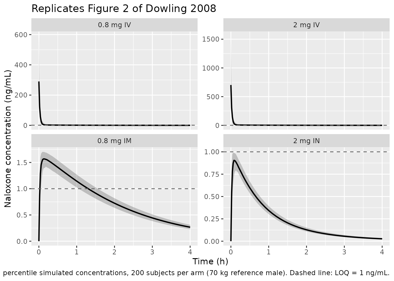
Figure 3: median concentration-time profiles across a dose range
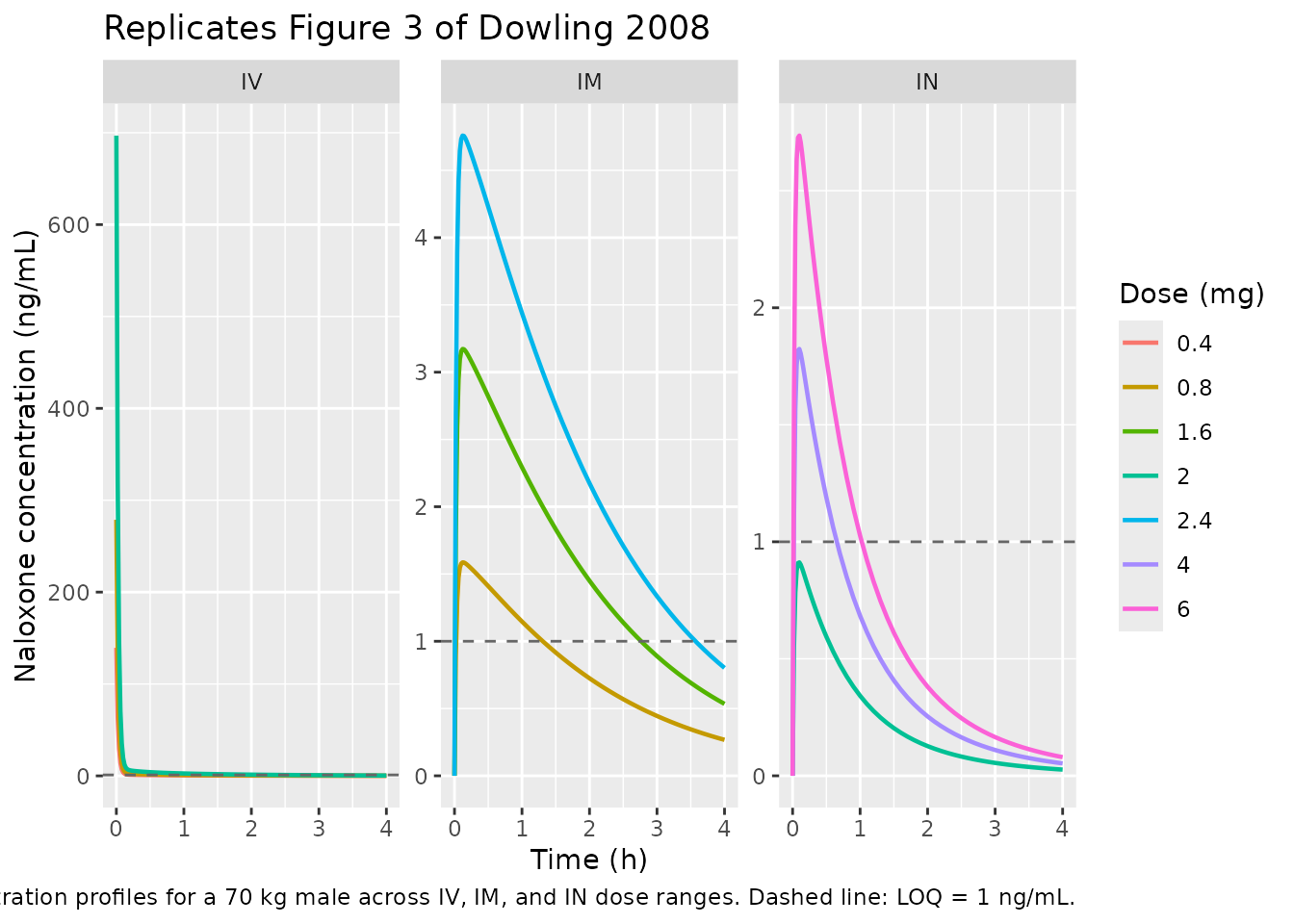
Dowling 2008 Figure 3 shows median concentration profiles for a range of IV (0.4, 0.8, 2 mg), IM (0.8, 1.6, 2.4 mg), and IN (2, 4, 6 mg) doses in 1000 70-kg subjects. The block below reproduces the same three panels using typical-value simulation (BSV zeroed) to match the paper’s median-only display.
mod_typical <- readModelDb("Dowling_2008_naloxone") |> rxode2::zeroRe()
#> ℹ parameter labels from comments will be replaced by 'label()'

fig3_arms <- tibble::tribble(
  ~route, ~dose_mg, ~cmt,
  "IV",   0.4,      "central",
  "IV",   0.8,      "central",
  "IV",   2.0,      "central",
  "IM",   0.8,      "depot",
  "IM",   1.6,      "depot",
  "IM",   2.4,      "depot",
  "IN",   2.0,      "depot2",
  "IN",   4.0,      "depot2",
  "IN",   6.0,      "depot2"
) |>
  dplyr::mutate(
    treatment = paste(dose_mg, "mg", route),
    route = factor(route, levels = c("IV", "IM", "IN"))
  )

fig3_events <- dplyr::bind_rows(lapply(seq_len(nrow(fig3_arms)), function(i) {
  row <- fig3_arms[i, ]
  tibble::tibble(
    id        = i,
    time      = c(0, obs_times),
    amt       = c(row$dose_mg, rep(NA_real_, length(obs_times))),
    evid      = c(1L, rep(0L, length(obs_times))),
    cmt       = c(row$cmt, rep("central", length(obs_times))),
    treatment = row$treatment,
    route     = as.character(row$route),
    dose_mg   = row$dose_mg,
    WT        = ref_wt_kg,
    FFM       = ref_ffm
  )
}))

sim_fig3 <- rxode2::rxSolve(
  mod_typical, events = fig3_events,
  keep = c("treatment", "route", "dose_mg")
) |>
  as.data.frame() |>
  dplyr::mutate(route = factor(route, levels = c("IV", "IM", "IN")))
#> ℹ omega/sigma items treated as zero: 'etalcl', 'etalvc'
#> Warning: multi-subject simulation without without 'omega'

ggplot(sim_fig3, aes(x = time, y = Cc, color = factor(dose_mg), group = treatment)) +
  geom_line(linewidth = 0.8) +
  geom_hline(yintercept = 1, linetype = "dashed", color = "grey40") +
  facet_wrap(~route, scales = "free_y") +
  labs(
    x = "Time (h)",
    y = "Naloxone concentration (ng/mL)",
    color = "Dose (mg)",
    title = "Replicates Figure 3 of Dowling 2008",
    caption = paste(
      "Typical-value (no IIV / no RUV) median concentration profiles",
      "for a 70 kg male across IV, IM, and IN dose ranges.",
      "Dashed line: LOQ = 1 ng/mL."
    )
  )
Numeric checks against Discussion prose (Tmax by route)
Dowling 2008 Results / Discussion quotes median time-to-peak concentration as 12 min for IM and 6-9 min for IN naloxone. The table below extracts Tmax from the typical-value simulations for the IM and IN Figure 3 arms and compares against the paper’s stated values.
tmax_by_arm <- sim_fig3 |>
  dplyr::filter(route %in% c("IM", "IN")) |>
  dplyr::group_by(treatment, route, dose_mg) |>
  dplyr::filter(!is.na(Cc)) |>
  dplyr::summarise(
    tmax_h   = time[which.max(Cc)],
    .groups = "drop"
  ) |>
  dplyr::mutate(
    tmax_min = tmax_h * 60,
    paper_min = dplyr::case_when(
      route == "IM" ~ "12",
      route == "IN" ~ "6-9"
    )
  ) |>
  dplyr::select(treatment, tmax_min, paper_min) |>
  dplyr::rename(
    "Treatment" = treatment,
    "Simulated Tmax (min)" = tmax_min,
    "Paper Tmax (min)"     = paper_min
  )

knitr::kable(
  tmax_by_arm,
  digits = 1,
  caption = paste(
    "Typical-value Tmax by dose group vs Dowling 2008 Results Section",
    "('median time to peak concentration for intramuscular naloxone ranged",
    "from 12 minutes and for intranasal from 6 to 9 minutes')."
  ),
  align = c("l", "r", "r")
)| Treatment | Simulated Tmax (min) | Paper Tmax (min) |
|---|---|---|
| 0.8 mg IM | 7.2 | 12 |
| 1.6 mg IM | 7.2 | 12 |
| 2 mg IN | 6.0 | 6-9 |
| 2.4 mg IM | 7.2 | 12 |
| 4 mg IN | 6.0 | 6-9 |
| 6 mg IN | 6.0 | 6-9 |
PKNCA validation
Single-dose NCA (0-4 h window) for each analyzable arm.
Concentrations from the stochastic VPC (sim) are used so
the per-arm summaries reflect the full between-subject distribution.
Time-zero anchor rows are added defensively; for extravascular routes
(IM, IN) pre-dose Cc = 0 is correct, and for the two IV arms the actual
t = 0 row is present in the observation grid so the
distinct() de-dup collapses the added row.
sim_nca <- sim |>
  dplyr::filter(!is.na(Cc)) |>
  dplyr::select(id, time, Cc, treatment)

sim_nca <- dplyr::bind_rows(
  sim_nca,
  sim_nca |>
    dplyr::distinct(id, treatment) |>
    dplyr::mutate(time = 0, Cc = 0)
) |>
  dplyr::distinct(id, treatment, time, .keep_all = TRUE) |>
  dplyr::arrange(id, treatment, time)

conc_obj <- PKNCA::PKNCAconc(
  sim_nca, Cc ~ time | treatment + id,
  concu = "ng/mL", timeu = "h"
)

dose_df <- events |>
  dplyr::filter(evid == 1L) |>
  dplyr::select(id, time, amt, treatment)

dose_obj <- PKNCA::PKNCAdose(
  dose_df, amt ~ time | treatment + id, doseu = "mg"
)

intervals <- data.frame(
  start      = 0,
  end        = 4,
  cmax       = TRUE,
  tmax       = TRUE,
  auclast    = TRUE,
  aucinf.obs = TRUE,
  half.life  = TRUE
)

nca_res <- PKNCA::pk.nca(
  PKNCA::PKNCAdata(conc_obj, dose_obj, intervals = intervals)
)

nca_summary <- as.data.frame(summary(nca_res))
knitr::kable(
  nca_summary,
  caption = paste0(
    "PKNCA summary (medians and 5th-95th percentiles) for each of the four ",
    "analyzable Dowling 2008 arms, over 0-4 h post-dose in a 70 kg reference cohort ",
    "of ", n_per_arm, " subjects per arm."
  )
)| Interval Start | Interval End | treatment | N | AUClast (h*ng/mL) | Cmax (ng/mL) | Tmax (h) | Half-life (h) | AUCinf,obs (h*ng/mL) |
|---|---|---|---|---|---|---|---|---|
| 0 | 4 | 0.8 mg IM | 200 | 3.20 [7.00] | 1.58 [5.61] | 0.120 [0.0600, 0.340] | 1.38 [0.0250] | 3.73 [7.64] |
| 0 | 4 | 0.8 mg IV | 200 | 10.0 [7.29] | 281 [49.2] | 0.000 [0.000, 0.000] | 1.08 [0.0241] | 10.3 [7.55] |
| 0 | 4 | 2 mg IN | 200 | 0.943 [7.68] | 0.910 [6.69] | 0.100 [0.0200, 0.220] | 0.970 [0.0298] | 0.981 [8.09] |
| 0 | 4 | 2 mg IV | 200 | 25.2 [7.28] | 702 [55.7] | 0.000 [0.000, 0.000] | 1.09 [0.0241] | 25.8 [7.53] |
Comparison against Dowling 2008 published values
Dowling 2008 does not report a full NCA table; the model-derived bioavailability values (F_im = 0.36 and F_in = 0.038) and the qualitative Tmax statements are the closest published anchors. The check below verifies dose-normalised AUC ratios against those two bioavailability values: IM/IV should be ~ 0.36 and IN/IV should be ~ 0.038 in a typical-value simulation.
# One typical-value subject per arm gives the same trajectory as the
# stochastic cohort (BSV zeroed via rxode2::zeroRe()) -- computing AUC on
# the single-subject sim is sufficient for the F cross-check.
typical_events <- dplyr::bind_rows(lapply(seq_len(nrow(arms)), function(i) {
  make_events_for_arm(arms[i, ], n = 1L, id_offset = (i - 1L))
}))

sim_typical_arms <- rxode2::rxSolve(
  mod_typical, events = typical_events, keep = c("treatment")
) |>
  as.data.frame() |>
  dplyr::filter(!is.na(Cc)) |>
  dplyr::mutate(treatment = factor(treatment, levels = arms$treatment))
#> ℹ omega/sigma items treated as zero: 'etalcl', 'etalvc'
#> Warning: multi-subject simulation without without 'omega'

auc_by_arm <- sim_typical_arms |>
  dplyr::arrange(treatment, time) |>
  dplyr::group_by(treatment) |>
  dplyr::summarise(
    auc0_4h = sum(diff(time) * (head(Cc, -1) + tail(Cc, -1)) / 2),
    .groups = "drop"
  ) |>
  dplyr::left_join(arms, by = "treatment") |>
  dplyr::mutate(dose_norm_auc = auc0_4h / dose_mg)

iv_08 <- auc_by_arm$dose_norm_auc[auc_by_arm$treatment == "0.8 mg IV"]
iv_2  <- auc_by_arm$dose_norm_auc[auc_by_arm$treatment == "2 mg IV"]
im_08 <- auc_by_arm$dose_norm_auc[auc_by_arm$treatment == "0.8 mg IM"]
in_2  <- auc_by_arm$dose_norm_auc[auc_by_arm$treatment == "2 mg IN"]

f_check <- tibble::tibble(
  Comparison             = c(
    "IM 0.8 mg AUC / IV 0.8 mg AUC",
    "IN 2 mg AUC / IV 2 mg AUC"
  ),
  simulated_F            = c(im_08 / iv_08, in_2 / iv_2),
  published_F            = c(0.36, 0.038)
) |>
  dplyr::mutate(
    rel_diff_pct = round(100 * (simulated_F - published_F) / published_F, 1)
  ) |>
  dplyr::rename(
    "Comparison"               = Comparison,
    "Simulated F (0-4 h AUC)"  = simulated_F,
    "Published F (Table 1)"    = published_F,
    "Rel. diff (%)"            = rel_diff_pct
  )

knitr::kable(
  f_check,
  digits = c(0, 3, 3, 1),
  caption = paste(
    "Dose-normalised AUC ratios from the typical-value simulation vs the",
    "F_im = 0.36 and F_in = 0.038 point estimates in Dowling 2008 Table 1.",
    "AUC computed over 0-4 h (matches the observation window)."
  ),
  align = c("l", "r", "r", "r")
)| Comparison | Simulated F (0-4 h AUC) | Published F (Table 1) | Rel. diff (%) |
|---|---|---|---|
| IM 0.8 mg AUC / IV 0.8 mg AUC | 0.308 | 0.360 | -14.5 |
| IN 2 mg AUC / IV 2 mg AUC | 0.036 | 0.038 | -5.3 |
Assumptions and deviations
- Race / ethnicity distribution not reported. The paper lists only n, sex, age, weight, and height; race / ethnicity is not stated. The virtual cohort therefore omits race indicators, matching the study’s covariate model (no race effects on any PK parameter).
-
Fat-free mass in the virtual cohort. Dowling 2008
uses
LBW2005, which the paper labels “lean body weight” but computes with the Janmahasatian et al. (2005) formula – biologically fat-free mass. The nlmixr2lib canonicalFFMis aligned with the Janmahasatian output; the model file’scovariateData$FFM$notesrecords the paper’sLBW2005naming choice. -
Reference weight of 70 kg for both allometric
terms. The paper’s final equations use
LBW2005 / 70andWT / 70even though the study’s median weight was 80 kg (n = 6, range 75-100). The 70 kg reference is the standard allometric anchor, and the packaged model preserves it verbatim. - Bioavailability point estimates only. Table 1 reports F_im = 0.36 (95% bootstrap 0.18-0.45) and F_in = 0.038 (0.016-0.040), the latter with a narrow interval because only two subjects had detectable IN concentrations after 2 mg. The packaged model uses the point estimates directly; downstream users simulating IN scenarios should treat the F_in estimate as an upper bound (Discussion / Limitations: “the bioavailability of 4% may be an overestimate and a more sensitive assay may allow a better estimate of the bioavailability”).
-
IV bioavailability set to 1 as structural anchor.
IV doses in the event table bypass the two absorption depots
(
cmt = "central"), so nof(central) <- ...assignment is needed and F_IV = 1 by construction, matching Methods ‘Data Analysis’ (“bioavailability was fixed to 1 for the intravenous route”). - BSV only on CL and V2. Table 1 and Results Section: “Addition of BSV on V3, V4, Q3, or Q4 did not reduce the objective function significantly or provided improbable estimates of BSV”; likewise BSV on Ka was tested for the IM route (more data than IN) but not retained. The packaged model omits BSV on the remaining structural parameters accordingly.
-
Between-occasion variability not modeled. Methods
‘Data Analysis’: “Between-occasion variability (intraindividual
variability) was not included in the modeling process because each
occasion represented a different dose or route of administration.” The
packaged model likewise has no
iov*parameters. -
LOQ handling. The paper set the first sub-LOQ
concentration per profile to LOQ / 2 = 0.5 ng/mL (Beal M3 alternative).
This affects the original fit but not the packaged forward simulation,
which returns model-predicted
Ccat every requested time. - Additive residual reported as fixed variance. Table 1 reports the additive error as 0.001 (fixed). Interpreted as NONMEM SIGMA (variance scale), giving SD = sqrt(0.001) = 0.0316 ng/mL – small compared to the 1 ng/mL LOQ. The proportional error 0.101 is likewise a variance; sqrt(0.101) = 0.318 matches the parenthetical 31.7% CV reported in Table 1.