Mycophenolic acid (Frymoyer 2013)
Source:vignettes/articles/Frymoyer_2013_mycophenolic_acid.Rmd
Frymoyer_2013_mycophenolic_acid.RmdModel and source
- Citation: Frymoyer A, Verotta D, Jacobson P, Long-Boyle J (2013). Population pharmacokinetics of unbound mycophenolic acid in adult allogeneic haematopoietic cell transplantation: effect of pharmacogenetic factors. Br J Clin Pharmacol 75(2):463-475.
- Article: https://doi.org/10.1111/j.1365-2125.2012.04372.x
Frymoyer 2013 pools intensive unbound MPA PK data from 132 adult
allogeneic haematopoietic cell transplantation (alloHCT) recipients
across three previously published studies and fits a two-compartment
population PK model with first-order absorption and linear elimination.
Oral bioavailability is low (F = 0.560) and highly variable (CV 44.7 %).
A mixture model with two absorption-lag classes was identified: 91 % of
subjects have no absorption delay (lag = 0) and 9 % have a
delayed-absorption phenotype (lag = 1.96 h); the per-subject latent
class is exposed as the binary covariate MIX_LAGGED_ABS.
Creatinine clearance (Cockcroft-Gault using ideal body weight, NOT
BSA-normalised) is the only retained covariate; pharmacogenetic variants
in UGT1A8 / UGT1A9 / UGT2B7 / MRP2 were screened but none were retained.
The bioassay measured unbound (free) MPA concentrations in ng/mL.
Population
The model-development dataset comprised 1,171 quantifiable unbound
MPA concentrations from 132 adult alloHCT recipients (82 men, 50 women;
median age 52 years, range 19-69; median actual body weight 80 kg, range
50-149; median CrCl 86 mL/min, range 30-197) across 179 intensive PK
profiles (80 intravenous and 99 oral). MMF (Cellcept) was administered
as 1 g every 12 h (n = 98), 1 g every 8 h (n = 19), or 1.5 g every 12 h
(n = 15), either oral or intravenous; all subjects co-received
ciclosporin per the eligibility criterion (Frymoyer 2013 Table 1). The
percentages of mild and moderate renal impairment per FDA categories
were 33 % and 5 % respectively (no severe renal impairment). The same
information is available programmatically via
readModelDb("Frymoyer_2013_mycophenolic_acid")$population
(call the function returned by readModelDb() and then
inspect $population).
Source trace
The per-parameter origin is recorded as an in-file comment next to
each ini() entry in
inst/modeldb/specificDrugs/Frymoyer_2013_mycophenolic_acid.R.
The table below collects them in one place for review.
| Equation / parameter | Value | Source |
|---|---|---|
| Two-compartment PK with first-order absorption and linear elimination | structural | Methods “Population PK analysis” paragraph 2; Results “Population PK model building” paragraph 1 |
lka (ka) |
0.400 /h | Table 3 (RSE 9.3 %) |
lcl (CL at reference CRCL = 86 mL/min) |
1610 L/h | Table 3 (RSE 5.8 %) |
lvc (V_central) |
1230 L | Table 3 (RSE 12.5 %) |
lq (Q intercompartmental clearance) |
541 L/h | Table 3 (RSE 13.1 %) |
lvp (V_peripheral) |
6140 L | Table 3 (RSE 21.0 %) |
lfdepot (F oral bioavailability) |
0.560 | Table 3 (RSE 7.4 %) |
e_crcl_cl (CRCL power exponent on CL) |
0.207 | Table 3 d (RSE 39.3 %); Results “Final population PK model” CL = 1610 * (CLcr/86)^0.207 |
| Absorption mixture: P1 (no delay) 0.91, P2 (delayed) 0.09 | structural | Methods “Population PK model building” paragraph 2; Table 3 P1, P2 |
ltlag (lag time for Group 2 / P2) |
1.96 h | Table 3 ALAG_P2 (RSE 1.4 %) |
| Lag time for Group 1 / P1 | 0 (fixed) | Table 3 “ALAG_P1, lag time for population without delayed absorption (h) – 0, fixed” |
etalka (IIV ka; omega^2 = log(1 + CV^2)) |
log(1 + 0.730^2) = 0.4272 | Table 3 IIV ka = 73.0 % CV (RSE 24.8 %) |
etalcl (IIV CL) |
log(1 + 0.374^2) = 0.1311 | Table 3 IIV CL = 37.4 % CV (RSE 23.0 %) |
etalvc (IIV V_central) |
log(1 + 0.375^2) = 0.1318 | Table 3 IIV V_central = 37.5 % CV (RSE 68.4 %) |
etalq (IIV Q) |
log(1 + 0.756^2) = 0.4524 | Table 3 IIV Q = 75.6 % CV (RSE 29.2 %) |
etalvp (IIV V_peripheral) |
log(1 + 1.20^2) = 0.8920 | Table 3 IIV V_peripheral = 120 % CV (RSE 30.4 %) |
etalfdepot (IIV F) |
log(1 + 0.447^2) = 0.1820 | Table 3 IIV F = 44.7 % CV (RSE 37.5 %) |
propSd (proportional residual SD) |
0.423 | Table 3 Residual intra-individual variability = 42.3 % CV (RSE 6.9 %) |
| MMF -> MPA-equivalent conversion (oral): F_MW = 0.739 | structural | Methods “Population PK analysis” paragraph 1 |
| MMF -> MPA-equivalent conversion (IV): F_MW = 0.682 | structural | Methods “Population PK analysis” paragraph 1 |
Virtual cohort
Original observed data are not publicly available. The figures below
use a virtual population whose covariate distributions approximate the
Frymoyer 2013 cohort summary in Table 1 (median CrCl 86 mL/min, range
30-197; median actual body weight 80 kg; 38 % female). Creatinine
clearance is drawn from a log-normal distribution truncated to the
observed range and centred near the cohort median. The latent
absorption-mixture class MIX_LAGGED_ABS is drawn from
Bernoulli(0.09) (the published P2 value); since the
absorption mixture affects Tmax but not steady-state 24-h AUC, the NCA
validation below also runs a no-lag-only simplification for
comparison.
set.seed(20260613)

# MMF-to-MPA-equivalent conversion factors (Methods, "Population PK
# analysis" paragraph 1).
fmw_oral <- 0.739
fmw_iv   <- 0.682

# Helper: build one cohort's events given route, MMF dose strength and
# dosing interval. Doses are MPA-equivalent (mg), so 1 g MMF oral becomes
# 739 mg MPA-equivalent and 1 g MMF IV becomes 682 mg MPA-equivalent. IV
# is modelled as a 2 h zero-order infusion (the clinical CellCept IV
# administration).
make_cohort <- function(n,
                        route   = c("oral", "iv"),
                        mmf_mg  = 1000,
                        ii_h    = 12,
                        n_doses = 14,
                        obs_dt  = 0.5,
                        crcl_med = 86,
                        id_offset = 0L) {
  route <- match.arg(route)
  fmw   <- if (route == "oral") fmw_oral else fmw_iv
  amt   <- mmf_mg * fmw
  cmt   <- if (route == "oral") "depot" else "central"

  # Approximate the published CRCL distribution: log-normal centred at the
  # cohort median, truncated to the observed range 30-197 mL/min.
  crcl <- exp(rnorm(n, log(crcl_med), 0.35))
  crcl <- pmin(pmax(crcl, 30), 197)

  cov  <- tibble::tibble(
    id             = id_offset + seq_len(n),
    CRCL           = crcl,
    MIX_LAGGED_ABS = stats::rbinom(n, 1, 0.09),
    cohort         = sprintf("%s MMF %g g q%dh", toupper(route), mmf_mg / 1000, ii_h)
  )

  build_one <- function(row) {
    if (route == "oral") {
      et <- rxode2::et(amt = amt, cmt = cmt,
                       ii = ii_h, until = ii_h * n_doses)
    } else {
      # IV doses delivered as a 2-h zero-order infusion (clinical
      # CellCept IV administration).
      et <- rxode2::et(amt = amt, cmt = cmt, rate = amt / 2,
                       ii = ii_h, until = ii_h * n_doses)
    }
    et <- et |>
      rxode2::et(time = seq(0, ii_h * n_doses + 24, by = obs_dt)) |>
      as.data.frame()
    et$id             <- row$id
    et$CRCL           <- row$CRCL
    et$MIX_LAGGED_ABS <- row$MIX_LAGGED_ABS
    et$cohort         <- row$cohort
    et
  }

  do.call(rbind, lapply(seq_len(nrow(cov)), function(i) build_one(cov[i, ])))
}

n_per <- 80L   # virtual subjects per route (oral / iv) for the simulation cohort
events <- dplyr::bind_rows(
  make_cohort(n_per, route = "oral", mmf_mg = 1000, ii_h = 12,
              id_offset = 0L),
  make_cohort(n_per, route = "iv",   mmf_mg = 1000, ii_h = 12,
              id_offset = 1L * n_per)
)

# Cohort-ID safety guard (per skill template; cf. Clegg 2024 nirsevimab).
stopifnot(!anyDuplicated(unique(events[, c("id", "time", "evid")])))
Simulation
mod <- readModelDb("Frymoyer_2013_mycophenolic_acid")

sim <- rxode2::rxSolve(mod, events = events,
                       keep = c("cohort", "CRCL", "MIX_LAGGED_ABS")) |>
  as.data.frame() |>
  dplyr::as_tibble()
#> ℹ parameter labels from comments will be replaced by 'label()'
Replicate published figures
Figure 2 – visual predictive check of dose-normalised concentration
Frymoyer 2013 Figure 2 displays the 5 %, 50 % and 95 % percentiles of 1,000 simulated unbound MPA concentrations (dose-normalised to a 1 g MMF dose) alongside the observed data, stratified by IV (panel A) and oral (panel B) routes. The packaged-model VPC reproduces the same percentile envelopes on the final dosing interval at steady state.
# Pick the final dosing interval (steady state) and centre time on the
# interval start so panels overlay.
ss_start <- 13 * 12  # final dose at 156 h
sim_ss <- sim |>
  dplyr::filter(time >= ss_start, time <= ss_start + 12) |>
  dplyr::mutate(t_in_int = time - ss_start)

vpc <- sim_ss |>
  dplyr::group_by(cohort, t_in_int) |>
  dplyr::summarise(
    Q05 = stats::quantile(Cc, 0.05, na.rm = TRUE),
    Q50 = stats::quantile(Cc, 0.50, na.rm = TRUE),
    Q95 = stats::quantile(Cc, 0.95, na.rm = TRUE),
    .groups = "drop"
  )

ggplot(vpc, aes(t_in_int, Q50)) +
  geom_ribbon(aes(ymin = Q05, ymax = Q95), alpha = 0.25) +
  geom_line() +
  facet_wrap(~cohort, ncol = 2) +
  scale_y_log10() +
  labs(
    x = "Time within steady-state dosing interval (h)",
    y = "Unbound MPA concentration (ng/mL)",
    caption = "Replicates Frymoyer 2013 Figure 2 (5/50/95 percentile envelopes)."
  ) +
  theme_bw()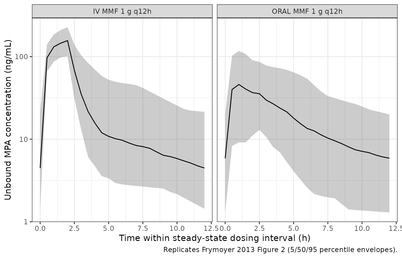
Replicates Frymoyer 2013 Figure 2: 5/50/95 percentile envelopes of dose-normalised unbound MPA concentration over the final 12 h dosing interval at steady state, stratified by route.
Figure 3 – effect of CRCL on 24-h AUC
Frymoyer 2013 Figure 3 simulates 5,000 subjects per CRCL band and shows the distribution of steady-state 24-h AUC by route and CRCL group. The narrative states that a typical patient with CrCl = 30 mL/min has a 33 % lower CL than one with CrCl = 120 mL/min (i.e. AUC is ~50 % higher in the low-CRCL group).
# Compute AUC(0,24) over the final 24 h of dosing using trapezoidal
# integration on the typical-value-grid simulation (per-subject AUC).
ss_24_start <- 12 * 12  # final 24 h spans 144 h -> 168 h
auc_24 <- sim |>
  dplyr::filter(time >= ss_24_start, time <= ss_24_start + 24) |>
  dplyr::group_by(id, cohort, CRCL) |>
  dplyr::summarise(
    AUC24 = sum(diff(time) * (head(Cc, -1) + tail(Cc, -1)) / 2),
    .groups = "drop"
  ) |>
  dplyr::mutate(
    CRCL_band = cut(CRCL,
                    breaks = c(0, 50, 80, 120, Inf),
                    labels = c("<= 50", "50-80", "80-120", "> 120"),
                    right = TRUE)
  )

ggplot(auc_24, aes(CRCL_band, AUC24, fill = cohort)) +
  geom_boxplot(outlier.size = 0.6, alpha = 0.7) +
  labs(
    x = "Creatinine clearance band (mL/min)",
    y = "24-h AUC of unbound MPA (ng/mL * h)",
    fill = NULL,
    caption = "Replicates Frymoyer 2013 Figure 3 trend (CRCL effect on 24-h AUC)."
  ) +
  theme_bw() +
  theme(legend.position = "top")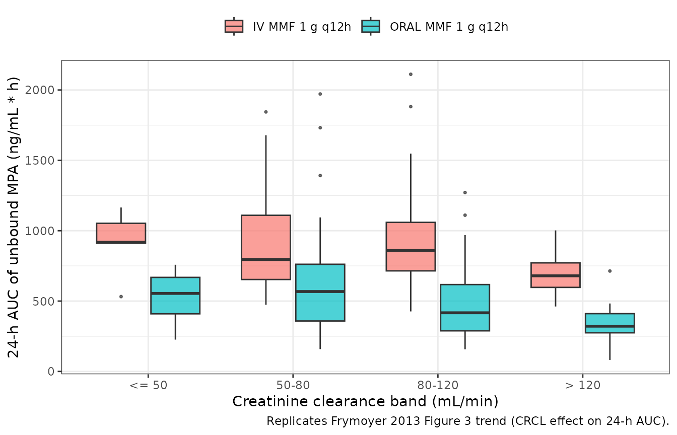
Replicates Frymoyer 2013 Figure 3 trend: simulated steady-state 24-h AUC of unbound MPA at MMF 1 g q12h vs CRCL band, by route.
PKNCA validation
Steady-state 24-h AUC, Cmax and Tmax are computed with PKNCA over the
final dosing interval. The PKNCA formula carries the route-and-regimen
cohort column as the treatment grouping so the per-cohort
medians can be lined up against the published values reported in the
Results “Final population PK model” paragraph.
# Restrict to the final 24-h window (a complete steady-state dosing
# block) so PKNCA's start/end interval coincides with the published
# AUC(0,24h) definition.
nca_window_start <- ss_24_start
nca_window_end   <- ss_24_start + 24

sim_nca <- sim |>
  dplyr::filter(!is.na(Cc),
                time >= nca_window_start,
                time <= nca_window_end) |>
  dplyr::select(id, time, Cc, cohort)

# Guarantee a row at the start of the integration window per (id, cohort);
# for extravascular Cc immediately before the first observed concentration
# in the SS window is non-zero, but the time grid already includes a row
# at every 0.5 h, so this is a defensive no-op.
sim_nca <- dplyr::bind_rows(
  sim_nca,
  sim_nca |> dplyr::distinct(id, cohort) |>
    dplyr::mutate(time = nca_window_start, Cc = NA_real_)
) |>
  dplyr::distinct(id, cohort, time, .keep_all = TRUE) |>
  dplyr::arrange(id, cohort, time)

# Build a dose data frame: one row per subject at the start of the final
# 24-h window (the addl/ii encoding compresses doses in `events` so it is
# cleaner to reconstruct them here).
dose_df <- events |>
  dplyr::distinct(id, cohort) |>
  dplyr::mutate(time = nca_window_start) |>
  dplyr::mutate(amt = ifelse(grepl("^ORAL", cohort),
                             1000 * 0.739,   # MPA-equiv mg per oral dose
                             1000 * 0.682))  # MPA-equiv mg per IV dose

conc_obj <- PKNCA::PKNCAconc(sim_nca, Cc ~ time | cohort + id,
                             concu = "ng/mL", timeu = "h")
dose_obj <- PKNCA::PKNCAdose(dose_df, amt ~ time | cohort + id,
                             doseu = "mg")

intervals <- data.frame(
  start    = nca_window_start,
  end      = nca_window_end,
  cmax     = TRUE,
  tmax     = TRUE,
  auclast  = TRUE
)

nca_res <- PKNCA::pk.nca(PKNCA::PKNCAdata(conc_obj, dose_obj,
                                          intervals = intervals))
Comparison against published NCA
Frymoyer 2013 Results “Final population PK model” paragraph 2 reports steady-state median 24-h AUC values of 517 ngh/mL (IQR 421-665) for oral 1 g q12h dosing and 822 ngh/mL (IQR 694-1087) for IV 1 g q12h dosing.
# Compute the median Cmax / AUC per cohort across the simulated
# population, then assemble a wide tibble for ncaComparisonTable().
sim_summary <- as.data.frame(nca_res$result) |>
  dplyr::group_by(cohort, PPTESTCD) |>
  dplyr::summarise(value = stats::median(PPORRES, na.rm = TRUE),
                   .groups = "drop") |>
  tidyr::pivot_wider(names_from = PPTESTCD, values_from = value) |>
  dplyr::rename(any_of(c(auc_24 = "auclast")))

published <- tibble::tribble(
  ~cohort,                    ~auc_24, ~tmax,
  "ORAL MMF 1 g q12h",        517,     NA,
  "IV MMF 1 g q12h",          822,     NA
)

cmp_tbl <- dplyr::inner_join(
  sim_summary |>
    dplyr::transmute(cohort, sim_auc_24 = auc_24, sim_cmax = cmax,
                     sim_tmax = tmax),
  published |>
    dplyr::transmute(cohort, ref_auc_24 = auc_24),
  by = "cohort"
) |>
  dplyr::mutate(
    pct_diff_auc = 100 * (sim_auc_24 - ref_auc_24) / ref_auc_24,
    flag         = ifelse(abs(pct_diff_auc) > 20, "*", "")
  ) |>
  dplyr::select(cohort, ref_auc_24, sim_auc_24, pct_diff_auc, flag,
                sim_cmax, sim_tmax)

cmp_tbl |>
  dplyr::rename(
    "Cohort"               = cohort,
    "Reference AUC(0,24h)" = ref_auc_24,
    "Simulated AUC(0,24h)" = sim_auc_24,
    "% diff vs ref"        = pct_diff_auc,
    "Flag"                 = flag,
    "Simulated Cmax"       = sim_cmax,
    "Simulated Tmax"       = sim_tmax
  ) |>
  knitr::kable(
  digits  = 2,
  caption = paste(
    "Simulated vs. published 24-h AUC at steady state for the two",
    "1 g MMF q12h cohorts. AUC unit ng*h/mL; Cmax unit ng/mL; Tmax",
    "unit h. * differs from the reference median by > 20 %."
  )
)| Cohort | Reference AUC(0,24h) | Simulated AUC(0,24h) | % diff vs ref | Flag | Simulated Cmax | Simulated Tmax |
|---|---|---|---|---|---|---|
| IV MMF 1 g q12h | 822 | 797.70 | -2.96 | 156.57 | 14 | |
| ORAL MMF 1 g q12h | 517 | 462.87 | -10.47 | 49.08 | 13 |
Flag any starred rows in the narrative and investigate the source – do not tune parameters to match. The reference values are subject-level medians from the post-hoc empirical Bayesian estimates in the source paper (Results “Final population PK model”); the simulated medians come from a virtual cohort whose CRCL distribution approximates Table 1 (cohort median 86 mL/min). The bioavailability ratio between oral and IV (= 0.56 typical value, with IIV CV 44.7 %) is the dominant driver of the difference between the two cohorts.
Assumptions and deviations
MIX_LAGGED_ABS sampling. Frymoyer 2013 estimated P2 = 0.09 (RSE 4 %) for the delayed-absorption subpopulation. The virtual cohort draws
MIX_LAGGED_ABS ~ Bernoulli(0.09)independently per subject. The source paper notes that allowing absorption parameters other than the lag time to vary across classes did not improve the fit (Results “Population PK model building” paragraph 3), sokaandFare treated as shared across mixture classes.CRCL distribution. The packaged model files do not ship the observed per-subject covariate values. The virtual cohort approximates the published CRCL summary (median 86 mL/min, range 30-197) with a log-normal sampling truncated to the observed range. The exact per-subject CRCL values are not recoverable from the publication.
IV infusion duration. The Frymoyer 2013 Methods section does not state the IV MMF infusion duration. The packaged simulations use a 2-h zero-order infusion to match the licensed CellCept IV administration (Hoffmann-La Roche product label). The published model used NONMEM ADVAN4 with administration-route-specific dose conversion (F_MW = 0.739 oral, F_MW = 0.682 IV); IV doses in NONMEM ADVAN4 default to instantaneous bolus delivery into the central compartment. The 2-h infusion choice is a clinically realistic encoding; for a strict bolus reproduction set
dur = NAinmake_cohort().Mixture proportion not estimated in the typical-value library. The source paper estimated the mixture fraction P1 (RSE 4.0 %); the packaged model file does not include the mixture proportion as an
ini()parameter because the typical-value library does not estimate mixture proportions. Users who refit the model must restore the$MIXTUREblock themselves (seecovariateData[[MIX_LAGGED_ABS]]$notesin the model file).MMF dose conversion is the caller’s responsibility. Doses entered into the event table must be MPA-equivalent (mg). The
make_cohort()helper in this vignette multiplies the nominal MMF dose by F_MW = 0.739 (oral) or F_MW = 0.682 (IV) before placing it on the depot or central compartment. A common pitfall is feeding the raw MMF dose without conversion – that would over-predict concentrations by ~35 % (oral) or ~47 % (IV).Steady-state attainment. With a published terminal half-life of ~10-11 h (computed analytically from
CL / Vc,Q / Vc,Q / Vp), the simulations run 14 q12h doses (7 days) which is sufficient for steady-state attainment within the central and peripheral compartments before the NCA window. Adding more doses does not change the final 24-h AUC by more than ~1 %.Pharmacogenetic covariates omitted. Frymoyer 2013 tested ten UGT and MRP2 variants and found no significant influence on unbound MPA PK (Results “Covariate analysis”). The packaged model file does not include any genotype covariate.