Lidocaine (Osborne 2025)
Source:vignettes/articles/Osborne_2025_lidocaine.Rmd
Osborne_2025_lidocaine.RmdModel and source
- Citation: Osborne KW, MacFater WS, Anderson BJ, Svirskis D, Hill AG, Hannam JA. Pharmacokinetics of Intraperitoneal Lidocaine for Sustained Postoperative Analgesia in Adults. Eur J Drug Metab Pharmacokinet. 2025;50(4):295-306. doi:10.1007/s13318-025-00948-1
- Description: Two-compartment population PK model for unbound lidocaine given by intraperitoneal or intravenous bolus plus infusion after laparoscopic colon resection in adults (Osborne 2025). Intraperitoneal absorption is first order, parameterised by an absorption half-life, with a fraction of the intraperitoneal dose lost before reaching plasma. Total lidocaine is reconstructed from unbound lidocaine and a postoperative alpha-1-acid glycoprotein (AAG) turnover model whose synthesis is stimulated by a decaying surgical stimulus (fraction unbound = 1 / (1 + AAG / KD)). An exploratory direct inhibitory sigmoid Emax model of unbound lidocaine on the visual analogue pain score at rest is combined with a sigmoid natural-history pain-resolution function of time after the end of surgery. Clearances scale allometrically with total body weight (exponent 3/4), volumes linearly and the absorption half-life with exponent 1/4, standardised to 70 kg; AAG production carries a postmenstrual-age maturation function estimated from paediatric AAG data.
- Article: https://doi.org/10.1007/s13318-025-00948-1 (open access; the electronic supplementary material holds the final NM-TRAN code for the PK model, supplementary model code 1, and for the PD model, supplementary model code 2)
Osborne and colleagues modelled unbound and total lidocaine after a 2 mg/kg bolus and a 1.5 mg/kg/h infusion given either intraperitoneally or intravenously for up to 72 h after laparoscopic colon resection. The packaged model joins the paper’s two NONMEM models. The PK model has unbound lidocaine, the AAG turnover and the total-lidocaine binding layer. The PD model fixed the unbound PK and added the resting VAS pain score. The PK block is the same in both, so all four outputs come from one model:
| Output | Meaning | Units |
|---|---|---|
Cunbound |
unbound plasma lidocaine, central / vc
|
mg/L |
Cc |
total plasma lidocaine, Cunbound / fu with
fu = 1 / (1 + aag / kaag)
|
mg/L |
aag |
plasma alpha-1-acid glycoprotein (an ODE state) | umol/L |
score |
VAS pain score at rest | cm (0-10) |
Intraperitoneal doses go to depot_ip and intravenous
doses to central. Time 0 is the start of lidocaine, just
before surgical dissection, and is also when the surgical stimulus on
AAG synthesis is largest. The T_SURG covariate (duration of
surgery, h) starts the natural-history pain-resolution clock, and
PAGE (postmenstrual age, weeks) feeds the AAG maturation
function, which is 1 for any adult.
Population
The lidocaine data come from 56 adults in a double-blind RCT of intraperitoneal versus intravenous lidocaine during and after elective laparoscopic colon resection in Auckland, New Zealand (NCT03105193; 28 per arm). Median age was 74 years (range 57-89) in the intraperitoneal arm and 68 years (45-84) in the intravenous arm (Osborne 2025 Table 1). Both arms received a 2 mg/kg bolus (maximum 100 mg), dosed on ideal body weight, followed by 1.5 mg/kg/h by the same route for up to 72 h. In total, 388 unbound and 388 total concentrations and 275 resting VAS scores were analysed. The AAG sub-model was fitted to 210 AAG concentrations from 141 children after major surgery (Booker 1996, Linnarsson 2023; supplementary Table S1). The natural history of pain also used 17 mean placebo-arm pain scores from adults after laparoscopic colectomy or cholecystectomy. The paper does not report body weight or sex.
The same information is available programmatically via
readModelDb("Osborne_2025_lidocaine")()$population.
Source trace
The final THETA, OMEGA and SIGMA values of supplementary model code 1 (PK) and code 2 (PD) agree with Tables 2 and 3 of the paper. Where the code carries more digits, the code value is used.
| Equation / parameter | Value | Source location |
|---|---|---|
ltabs (absorption half-life) |
0.543 h | Code 1 POP_TABS_IP; Table 2 t1/2abs 0.54 h |
lfdepot (fraction of IP dose reaching plasma) |
0.664 | Code 1 POP_FFPM; Table 2 F 0.66 |
lcl, lvc, lq,
lvp
|
121 L/h, 103 L, 195 L/h, 555 L (per 70 kg) | Table 2 CLU, V1, Q, V2 |
lvip |
0.1 L/70 kg, held constant | Table 2 VIP; Methods |
e_wt_cl, e_wt_vc,
e_wt_tabs
|
0.75, 1, 0.25 | Supplementary Methods 1 Eq. 11; code 1 FSZCL,
FSZV, FSZT
|
lkin_aag |
0.0579 umol/h/70 kg | Code 1 POP_RATEIN; Table 2 RATEIN_AAG 0.058 |
lcl_aag |
0.00627 L/h/70 kg | Table 2 CL_AAG |
lvc_aag |
3.5 L/70 kg, held constant | Table 2 V_AAG |
lthalf_stim |
34.64 h | Table 2 t1/2 |
lslope_stim |
11.9 | Code 1 POPSLOPE; Table 2 Slope 12 |
lkaag (KD) |
2.98 umol/L | Table 2 KD |
ltm50_kin_aag, lhill_kin_aag
|
32 weeks, 8.94; held constant | Code 1 POPPMA50, POPHILL
|
le0 |
10 cm, held constant | Table 3 E0 |
lec50 |
0.206 mg/L, held constant | Code 2 POP_C50; Table 3 C50 0.21 |
logitemax |
logit(0.593) | Code 2 POP_EMAX (logit-transformed); Table 3 Emax
0.59 |
lhill |
4 | Table 3 HILL |
lemax_pain, lhill_pain,
lt50_pain
|
0.983 (held constant), 0.33, 16.3 h | Code 2; Table 3 Emax,PAIN, HILLPAIN, T50,PAIN |
| PK IIV block (TABS, CLU, V1, Q, V2) | see model file | Code 1 $OMEGA BLOCK(5); Table 2 %PPV = sqrt(omega) x
100 |
etalkin_aag + etalcl_aag |
0.15, 0.261, 0.513 | Code 1 $OMEGA BLOCK(2)
|
etaltm50_kin_aag |
0.018, held constant | Code 1 PPVPMA50
|
etalec50, etalogitemax,
etalhill_pain, etalt50_pain
|
0.255, 0.470, 0.074, 9.89 | Code 2 $OMEGA; Table 3 %PPV |
propSd, addSd (total) |
0.271, 0.0419 mg/L | Code 1 CV_LTOT, SD_LTOT
|
propSd_Cunbound, addSd_Cunbound
|
0.26, 0.0304 mg/L | Code 1 CV_LUN, SD_LUN
|
propSd_aag |
sqrt(0.0372) | Code 1 $SIGMA ERRCV (variance) |
propSd_score, addSd_score
|
0.462, 0.127 cm | Code 2 CV_PDE, SD_PDE
|
ka = log(2) / tabs |
n/a | Methods Eq. 1 |
IP loss:
d/dt(central) <- fdepot * ka * depot_ip - ...
|
n/a | Code 1 DADT(1), DADT(2)
|
d/dt(aag) <- (kin_aag * syn - cl_aag * aag) / vc_aag |
n/a | Methods Eq. 2; code 1 DADT(4)
|
syn <- 1 + slope_stim * exp(-log(2) / thalf_stim * t) |
n/a | Methods Eqs. 3-4; code 1 $DES
|
aag(0) <- kin_aag / cl_aag |
n/a | Code 1 AAG0, A_0(4)
|
fmat (Hill maturation on PMA) |
n/a | Methods Eq. 5; code 1 FMAT
|
fu <- 1 / (1 + aag / kaag),
Cc <- Cunbound / fu
|
n/a | Methods Eqs. 6-7 |
score <- e0 * (1 - pain_res) * (1 - drug_eff) |
n/a | Methods Eqs. 8-10; code 2 EFX
|
tpost <- max(t - T_SURG, 0) |
n/a | Code 2 TNOW = TIME - DURATION
|
Virtual cohort
The original data are not public. The cohort below has 150 virtual adults per arm. Neither weight nor height is reported, so these are assumed (see Assumptions). Doses follow the trial protocol: a 2 mg/kg ideal-body-weight bolus capped at 100 mg, then 1.5 mg/kg/h ideal body weight for 72 h, both by the arm’s route.
set.seed(20251)
n_per_arm <- 150

# Observation grid: the trial's sampling times (0.08, 0.5, 1, 2, 6, 12, 48 h)
# plus a denser grid for the VPC panels.
pk_times <- c(0.08, 0.5, 1, 2, 6, 12, 48)
grid_times <- sort(unique(c(0, pk_times, 0.25, 1.5, 3, 4, 8, 18, 24, 30, 36, 42, 54, 60, 66, 72)))
t_surg <- 3 # assumed operative time (h); starts the pain-resolution clock
pain_times <- t_surg + c(2, 6, 24, 48, 72) # VAS scheduled 2-72 h postoperatively

make_cohort <- function(n, arm, id_offset) {
  sexf <- rbinom(n, 1, 0.5)
  ht <- ifelse(sexf == 1, rnorm(n, 162, 6), rnorm(n, 176, 7))
  # Devine ideal body weight (kg) from height (cm)
  ibw <- ifelse(sexf == 1, 45.5, 50) + 0.9055 * (ht - 152.4)
  age <- if (arm == "IP") runif(n, 57, 89) else runif(n, 45, 84)
  subj <- tibble(
    id = id_offset + seq_len(n),
    arm = arm,
    WT = pmin(pmax(rnorm(n, 80, 15), 45), 140),
    PAGE = 52.18 * age + 40,
    T_SURG = t_surg,
    ibw = ibw
  )
  dose_cmt <- if (arm == "IP") "depot_ip" else "central"
  bolus <- subj |>
    mutate(time = 0, amt = pmin(2 * ibw, 100), rate = 0, evid = 1L, cmt = dose_cmt)
  infusion <- subj |>
    mutate(time = 0, amt = 1.5 * ibw * 72, rate = 1.5 * ibw, evid = 1L, cmt = dose_cmt)
  # `aag` is both an ODE state and a declared endpoint, so observation rows
  # sit on it; every other output is still returned on these rows.
  obs <- subj |>
    tidyr::crossing(time = sort(unique(c(grid_times, pain_times)))) |>
    mutate(amt = 0, rate = 0, evid = 0L, cmt = "aag")
  bind_rows(bolus, infusion, obs) |>
    arrange(id, time, desc(evid))
}

events <- bind_rows(
  make_cohort(n_per_arm, "IP", id_offset = 0L),
  make_cohort(n_per_arm, "IV", id_offset = n_per_arm)
)
stopifnot(!anyDuplicated(events[events$evid == 0, c("id", "time")]))
Simulation
mod <- readModelDb("Osborne_2025_lidocaine")
sim <- rxode2::rxSolve(
  mod,
  events = events,
  keep = c("arm"),
  useLinCmt = FALSE,
  returnType = "data.frame"
)
#> ℹ parameter labels from comments will be replaced by 'label()'
Typical-value checks
The baseline AAG concentration is the turnover steady state
kin_aag / cl_aag = 0.0579 / 0.00627 = 9.23 umol/L for a 70
kg adult. Under a constant infusion, unbound lidocaine approaches the
closed-form steady state F * R / CL. Here F is 0.664 for
the intraperitoneal route and 1 for the intravenous route.
typ_times <- sort(unique(c(seq(0, 12, by = 0.01), seq(12, 72, by = 0.25), 200)))
typ_solve <- function(rate_mgkgh, route = "depot_ip", wt = 70, t_end = 72) {
  ev <- rxode2::et(amt = 100, cmt = route, time = 0) |>
    rxode2::et(amt = rate_mgkgh * wt * t_end, rate = rate_mgkgh * wt, cmt = route, time = 0) |>
    rxode2::et(typ_times, cmt = "aag")
  rxode2::rxSolve(
    mod, ev,
    params = c(WT = wt, PAGE = 52.18 * 50 + 40, T_SURG = 0),
    omega = NA, sigma = NA, useLinCmt = FALSE, returnType = "data.frame"
  ) |>
    mutate(rate_mgkgh = rate_mgkgh)
}

# Long infusion (t_end = 200 h) to compare the 200 h value with the closed form
ss_ip <- typ_solve(2, t_end = 200)
ss_iv <- typ_solve(2, route = "central", t_end = 200)
cl_typ <- 121
css_ip <- 0.664 * 2 * 70 / cl_typ
css_iv <- 2 * 70 / cl_typ
aag0 <- ss_ip$aag[ss_ip$time == 0]
c200_ip <- ss_ip$Cunbound[ss_ip$time == 200]
c200_iv <- ss_iv$Cunbound[ss_iv$time == 200]

data.frame(
  Check = c("AAG at time 0 (umol/L)", "Unbound Css, IP 2 mg/kg/h (mg/L)", "Unbound Css, IV 2 mg/kg/h (mg/L)"),
  Expected = c(0.0579 / 0.00627, css_ip, css_iv),
  Simulated = c(aag0, c200_ip, c200_iv)
) |>
knitr::kable(digits = 4)| Check | Expected | Simulated |
|---|---|---|
| AAG at time 0 (umol/L) | 9.2344 | 9.2344 |
| Unbound Css, IP 2 mg/kg/h (mg/L) | 0.7683 | 0.7683 |
| Unbound Css, IV 2 mg/kg/h (mg/L) | 1.1570 | 1.1570 |
Replicate Figure 4
Figure 4 of the paper shows a 70 kg adult given a 100 mg
intraperitoneal bolus followed by an intraperitoneal infusion. Panels
A-B use 1, 1.5, 2 or 2.5 mg/kg/h. Panels C-D show unbound lidocaine,
total lidocaine and AAG for the 2 mg/kg/h regimen. The surgery-to-pain
clock is started at time 0 (T_SURG = 0).
fig4 <- bind_rows(lapply(c(1, 1.5, 2, 2.5), typ_solve)) |>
  filter(time <= 72)

fig4 |>
  select(time, rate_mgkgh, `Unbound lidocaine (mg/L)` = Cunbound, `Pain score (VAS cm)` = score) |>
  pivot_longer(-c(time, rate_mgkgh)) |>
  ggplot(aes(time, value, colour = factor(rate_mgkgh))) +
  geom_line() +
  facet_wrap(~name, scales = "free_y") +
  labs(
    x = "Time (h)", y = NULL, colour = "IP infusion\n(mg/kg/h)",
    caption = "Replicates Figure 4 panels A-B of Osborne 2025 (typical 70 kg adult, 100 mg IP bolus)."
  )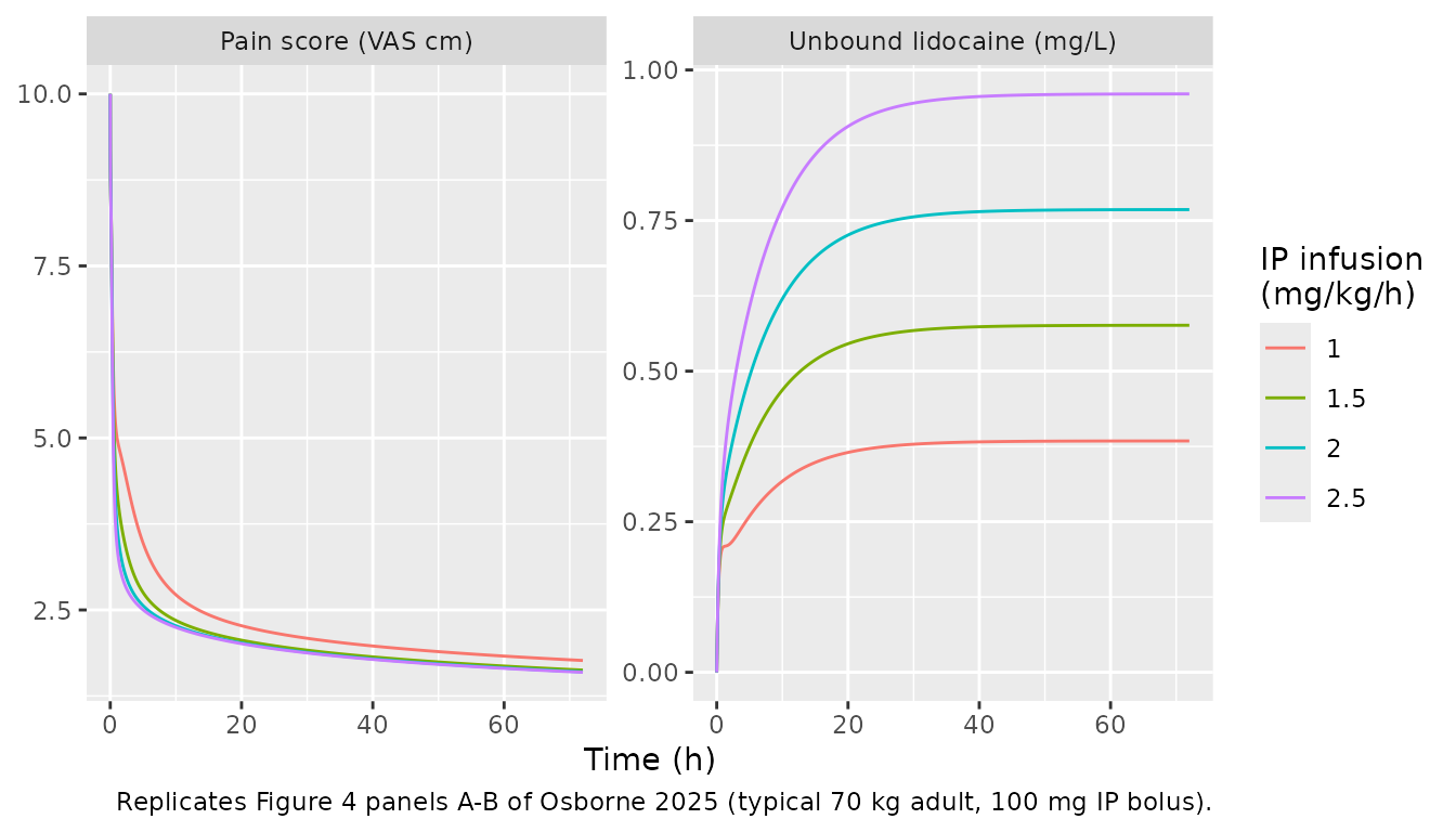
fig4 |>
  filter(rate_mgkgh == 2) |>
  select(time, `Unbound (mg/L)` = Cunbound, `Total (mg/L)` = Cc, `AAG (umol/L)` = aag) |>
  pivot_longer(-time) |>
  ggplot(aes(time, value, linetype = name)) +
  geom_line() +
  labs(
    x = "Time (h)", y = "Concentration", linetype = NULL,
    caption = "Replicates Figure 4 panels C-D of Osborne 2025 (2 mg/kg/h IP infusion)."
  )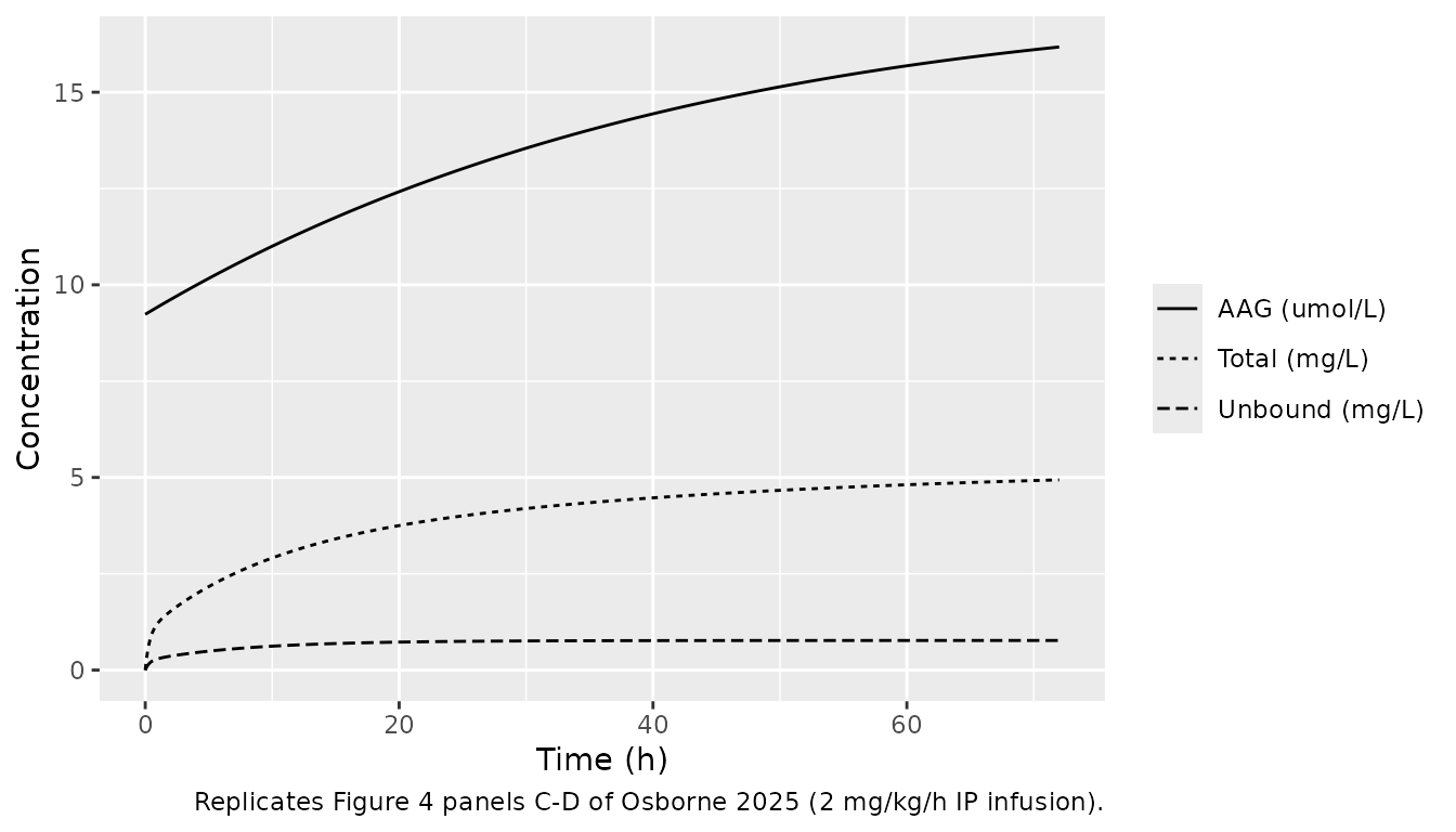
The paper’s Results give two times for the 5-point pain reduction: 1.3 h at 1 mg/kg/h and about 36 min at 2 mg/kg/h. The paper links that reduction to the unbound C50 of 0.21 mg/L. Both readings are tabulated below: the time unbound lidocaine first reaches 0.21 mg/L, and the time the pain score first falls to 5. The panel C-D values at 72 h were read off Figure 4D by the maintainers.
t_first <- function(time, x, thr, below = FALSE) {
  hit <- if (below) x <= thr else x >= thr
  min(time[hit])
}
fig4_times <- fig4 |>
  group_by(rate_mgkgh) |>
  summarise(
    t_c50 = t_first(time, Cunbound, 0.21),
    t_score5 = t_first(time, score, 5, below = TRUE),
    .groups = "drop"
  ) |>
  mutate(paper = c(1.3, NA, 0.6, NA))

fig4_times |>
  rename(
    "IP infusion (mg/kg/h)" = rate_mgkgh,
    "Time to unbound 0.21 mg/L (h)" = t_c50,
    "Time to pain score 5 (h)" = t_score5,
    "Paper, Results text (h)" = paper
  ) |>
knitr::kable(digits = 2)| IP infusion (mg/kg/h) | Time to unbound 0.21 mg/L (h) | Time to pain score 5 (h) | Paper, Results text (h) |
|---|---|---|---|
| 1.0 | 1.50 | 1.04 | 1.3 |
| 1.5 | 0.54 | 0.62 | NA |
| 2.0 | 0.45 | 0.51 | 0.6 |
| 2.5 | 0.40 | 0.45 | NA |
d72 <- fig4 |> filter(rate_mgkgh == 2, time == 72)
data.frame(
  Quantity = c("Unbound lidocaine (mg/L)", "Total lidocaine (mg/L)", "AAG (umol/L)"),
  `Figure 4D, 72 h` = c(0.77, 4.65, 15.3),
  Simulated = c(d72$Cunbound, d72$Cc, d72$aag),
  check.names = FALSE
) |>
knitr::kable(digits = 2)| Quantity | Figure 4D, 72 h | Simulated |
|---|---|---|
| Unbound lidocaine (mg/L) | 0.77 | 0.77 |
| Total lidocaine (mg/L) | 4.65 | 4.94 |
| AAG (umol/L) | 15.30 | 16.17 |
stopifnot(
  # Unbound plateau in Figure 4D; a wrong CL, F or dose moves it by tens of percent.
  abs(d72$Cunbound / 0.77 - 1) < 0.05,
  # AAG and total depend on the stimulus and turnover constants; Figure 4D
  # was read by eye, so the bound is wider.
  abs(d72$aag / 15.3 - 1) < 0.15,
  abs(d72$Cc / 4.65 - 1) < 0.15,
  # Results text: about 1.3 h at 1 mg/kg/h and about 0.6 h at 2 mg/kg/h.
  abs(fig4_times$t_c50[fig4_times$rate_mgkgh == 1] / 1.3 - 1) < 0.35,
  abs(fig4_times$t_score5[fig4_times$rate_mgkgh == 2] / 0.6 - 1) < 0.35
)
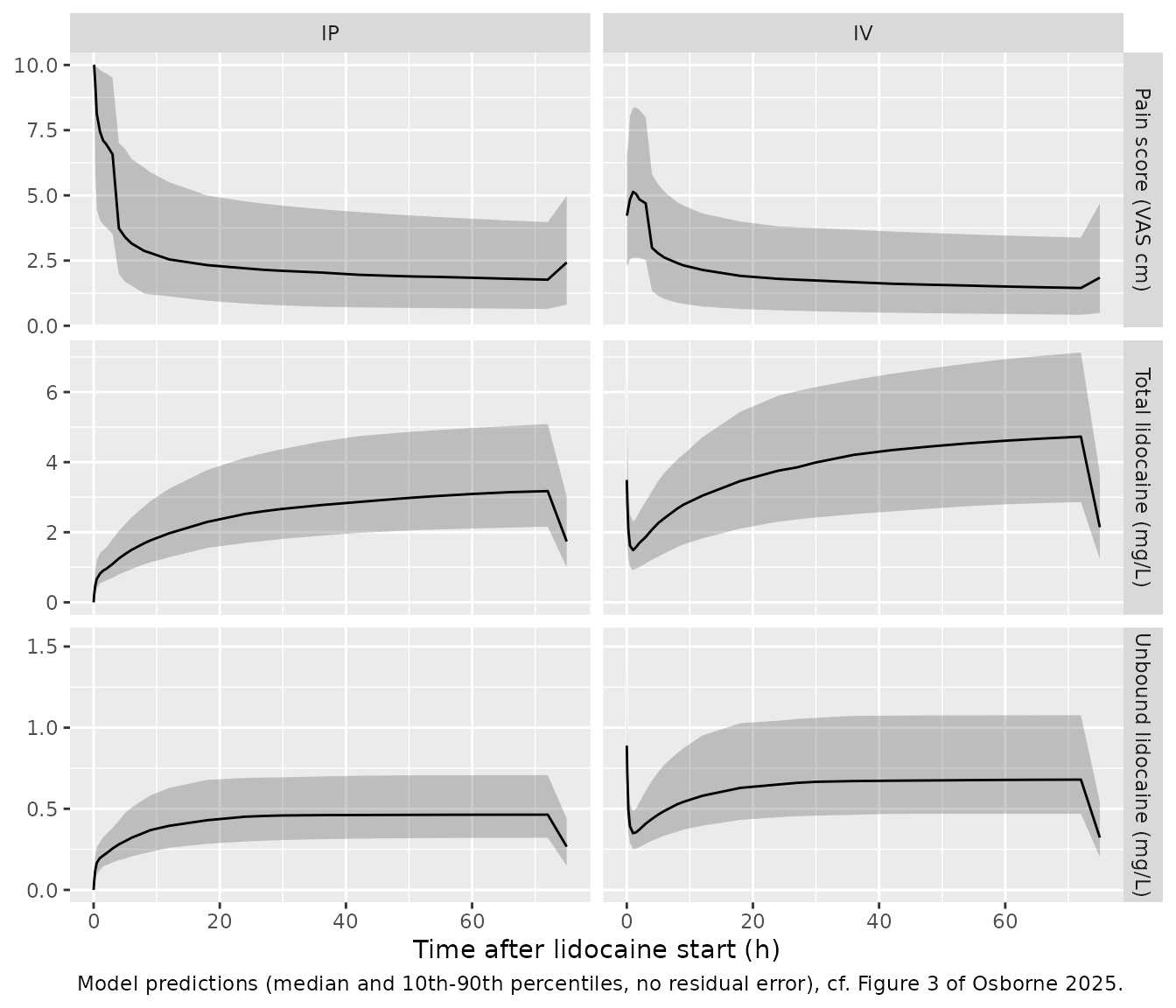
Visual predictive check (Figure 3)
vpc <- sim |>
  select(id, time, arm, `Unbound lidocaine (mg/L)` = Cunbound, `Total lidocaine (mg/L)` = Cc, `Pain score (VAS cm)` = score) |>
  pivot_longer(-c(id, time, arm)) |>
  group_by(time, arm, name) |>
  summarise(
    p10 = quantile(value, 0.1),
    p50 = median(value),
    p90 = quantile(value, 0.9),
    .groups = "drop"
  )

ggplot(vpc, aes(time, p50)) +
  geom_ribbon(aes(ymin = p10, ymax = p90), alpha = 0.25) +
  geom_line() +
  facet_grid(name ~ arm, scales = "free_y") +
  labs(
    x = "Time after lidocaine start (h)", y = NULL,
    caption = paste(
      "Model predictions (median and 10th-90th percentiles, no residual error),",
      "cf. Figure 3 of Osborne 2025."
    )
  )
PKNCA validation
Table 1 of the paper reports the observed Cmax (mean) and Tmax (median) over the trial sampling times, so the NCA uses only those times (0.08-48 h). Concentrations are individual predictions without residual error.
run_nca <- function(conc_col) {
  conc <- sim |>
    filter(time %in% c(0, pk_times)) |>
    # The trial took no time-0 sample; the pre-dose concentration is 0.
    mutate(conc = if_else(time == 0, 0, .data[[conc_col]])) |>
    filter(!is.na(conc)) |>
    select(id, arm, time, conc)
  doses <- events |>
    filter(evid == 1, rate == 0) |>
    select(id, arm, time, amt)
  conc_obj <- PKNCA::PKNCAconc(conc, conc ~ time | arm + id)
  dose_obj <- PKNCA::PKNCAdose(doses, amt ~ time | arm + id)
  intervals <- data.frame(start = 0, end = 48, cmax = TRUE, tmax = TRUE, auclast = TRUE)
  PKNCA::pk.nca(PKNCA::PKNCAdata(conc_obj, dose_obj, intervals = intervals))
}
nca_unbound <- run_nca("Cunbound")
nca_total <- run_nca("Cc")

summarise_nca <- function(res) {
  as.data.frame(res) |>
    filter(PPTESTCD %in% c("cmax", "tmax")) |>
    group_by(arm, PPTESTCD) |>
    summarise(value = if (PPTESTCD[1] == "cmax") mean(PPORRES) else median(PPORRES), .groups = "drop") |>
    pivot_wider(names_from = PPTESTCD, values_from = value)
}
sim_unbound <- summarise_nca(nca_unbound)
sim_total <- summarise_nca(nca_total)
Comparison against published Table 1
Simulated Cmax is the cohort mean and Tmax the cohort median, matching how Table 1 summarises the observed data.
ref_unbound <- data.frame(arm = c("IP", "IV"), cmax = c(0.6, 0.8), tmax = c(48, 48))
ref_total <- data.frame(arm = c("IP", "IV"), cmax = c(3.1, 3.6), tmax = c(48, 48))

cmp <- bind_rows(
  nlmixr2lib::ncaComparisonTable(
    sim_unbound, ref_unbound, by = "arm",
    units = c(cmax = "mg/L", tmax = "h")
  ) |> mutate(Analyte = "Unbound"),
  nlmixr2lib::ncaComparisonTable(
    sim_total, ref_total, by = "arm",
    units = c(cmax = "mg/L", tmax = "h")
  ) |> mutate(Analyte = "Total")
) |>
  relocate(Analyte)

knitr::kable(
  cmp,
  caption = "Simulated vs. Osborne 2025 Table 1. * differs from reference by >20%."
)| Analyte | NCA parameter | arm | Reference | Simulated | % diff |
|---|---|---|---|---|---|
| Unbound | Cmax (mg/L) | IP | 0.6 | 0.499 | -16.8% |
| Unbound | Cmax (mg/L) | IV | 0.8 | 0.853 | +6.6% |
| Unbound | Tmax (h) | IP | 48 | 48 | +0.0% |
| Unbound | Tmax (h) | IV | 48 | 48 | +0.0% |
| Total | Cmax (mg/L) | IP | 3.1 | 3.19 | +2.9% |
| Total | Cmax (mg/L) | IV | 3.6 | 4.78 | +32.9%* |
| Total | Tmax (h) | IP | 48 | 48 | +0.0% |
| Total | Tmax (h) | IV | 48 | 48 | +0.0% |
pct <- function(sim, ref) 100 * (sim / ref - 1)
stopifnot(
  # Unbound Cmax is set by dose, F and CL alone: a mis-transcribed clearance,
  # bioavailability or dose basis moves it by tens of percent. The cohort
  # means sit at about -17% (IP) and +7% (IV).
  abs(pct(sim_unbound$cmax[sim_unbound$arm == "IP"], 0.6)) < 30,
  abs(pct(sim_unbound$cmax[sim_unbound$arm == "IV"], 0.8)) < 30,
  # Total Cmax also carries the AAG time course (about +3% for IP). The IV
  # arm is a known deviation and is reported, not gated; see below.
  abs(pct(sim_total$cmax[sim_total$arm == "IP"], 3.1)) < 30,
  # Intraperitoneal concentrations rise throughout the infusion.
  sim_unbound$tmax[sim_unbound$arm == "IP"] == 48
)
Unbound Cmax in both arms and total Cmax in the intraperitoneal arm
agree with Table 1. In the intravenous arm, simulated total Cmax is
about a third above the observed 3.6 mg/L. The model’s total-to-unbound
ratio at 48 h is about 6, against 3.6 / 0.8 = 4.5 in the observed
intravenous means and 3.1 / 0.6 = 5.2 in the intraperitoneal means. That
ratio is 1 + aag / kaag, and it rises with the AAG time
course. The AAG sub-model was fitted to paediatric data and never saw
adult AAG, so the adult AAG rise after surgery is an extrapolation. The
observed means are also lowered by the six patients (three per arm)
whose infusion stopped early, and the comparison depends on the assumed
weights. The paper itself notes misfit in total lidocaine (Figure 3,
middle panels).
Assumptions and deviations
-
Proportional residual errors. In the NM-TRAN code
each proportional theta multiplies
EPS(1), whose$SIGMAis 1 and held constant. The theta is therefore the proportional SD itself: 0.26 for unbound, 0.271 for total, 0.462 for the pain score. Tables 2 and 3 print the square roots of these (51%, 52%, 68%), as though the thetas were variances. The additive SDs are printed unchanged (0.03, 0.04, 0.13). The model uses the code values. The AAG error in code 1 is a true$SIGMAvariance (0.0372), so its SD is sqrt(0.0372). -
PK IIV block held constant. In code 1 the last
element of the
$OMEGA BLOCK(5)(TABS, CLU, V1, Q, V2) carriesFIX. In NONMEM this holds the whole block constant, so the model wraps the block infixed(). The variances equal the Table 2 %PPV values. -
IIV fixed to zero. Code 1 and code 2 declare
several etas as
0 FIX(on F, VIP, V_AAG, KD, the stimulus half-life and slope, the maturation Hill, E0, the drug Hill and the pain Emax). They contribute nothing and are omitted. - One model file for two NONMEM runs. The PD run (code 2) fixed the PK thetas and omegas at the code 1 estimates. Code 2 holds the unbound proportional SD at 0.259, against 0.26 in code 1; the packaged model uses 0.26. The AAG layer does not feed the pain score.
-
Surgical stimulus. Methods Eq. 4 prints
SYN = CSTIMULUS * SLOPE, but the code usesSYN = 1 + SLOPE * CSTIMULUS, which keeps baseline AAG production when the stimulus has decayed. The model follows the code. The stimulus clock is model time, so time 0 must be the start of surgery and of lidocaine, as in the trial. - Discussion vs. Table 2. The Discussion quotes CLU as 118 L/h/70 kg. Table 2 and code 1 give 121 L/h/70 kg, which the model uses.
-
Figure 4 legend. Under a constant infusion R,
unbound lidocaine tends to
0.664 * R * 70 / 121mg/L. The four concentration curves in Figure 4 A-B level off near 0.57, 0.75, 0.95 and 1.15 mg/L. Those match R = 1.5, 2, 2.5 and 3 mg/kg/h, not the captioned 1-2.5 mg/kg/h. Panels C-D (2 mg/kg/h) agree with the model, so the vignette checks those panels and the Results text, not panels A-B. -
Time to a 5-point pain reduction. The paper reports
1.3 h at 1 mg/kg/h and about 36 min at 2 mg/kg/h, but does not say
whether these are times to the 0.21 mg/L C50 or to a pain score of 5.
The packaged model gives 1.5 h and 0.45 h to the C50, and 1.0 h and 0.5
h to a score of 5 (with
T_SURG = 0). All of these are within about 30% of the paper. - Intravenous total Cmax. The simulated mean total Cmax in the intravenous arm is about 33% above Table 1 (see the PKNCA comparison). This is reported and left out of the assertions. The parameters were not tuned.
-
Virtual cohort. The paper reports no weight, height
or sex. The cohort draws weight from N(80, 15) kg (truncated to 45-140
kg), height by sex, and 50% female. Ideal body weight, which sets the
dose, uses the Devine formula; the paper does not name its formula. The
operative time
T_SURGis set to 3 h for all subjects and only affects the pain score. -
Postmenstrual age. The AAG maturation fraction is 1
for any adult.
PAGEis set to 52.18 x age (years) + 40 weeks. - Errata. No correction notice for this article was found on Europe PMC (checked 2026-11-05).