Levosimendan (Bertin 2026)
Source:vignettes/articles/Bertin_2026_levosimendan.Rmd
Bertin_2026_levosimendan.RmdModel and source
- Citation: Bertin S, Guidi M, Haefliger D, Thoueille P, Bardinet C, Decosterd LA, Perez MH, Giraud R, Assouline B, Schneider A, Buclin T, Livio F. Population pharmacokinetics of levosimendan and its metabolites OR-1855 and OR-1896 in critically ill adults, neonates and infants on veno-arterial ECMO. Clin Pharmacokinet. 2026;65:XX. doi:10.1007/s40262-025-01591-4. Parameter values are the full-precision final estimates taken from the NONMEM control stream reproduced in Electronic Supplementary Material ‘Supplementary 10: NONMEM code for final model’, cross-checked against Table 2 of the main paper (which rounds several of them).
- Description: Joint parent-metabolite population PK model for intravenous levosimendan and its metabolites OR-1855 (inactive) and OR-1896 (active, long-lasting) in critically ill adults, neonates and infants supported by veno-arterial extracorporeal membrane oxygenation (VA-ECMO). Levosimendan disposition is two-compartment with first-order elimination; a single transit compartment carries the delayed formation of OR-1855, with the rate constant for entering the transit compartment set equal to the rate constant for leaving it. OR-1855 is either eliminated or acetylated to OR-1896, which is in turn eliminated or deacetylated back to OR-1855. Both metabolites are assumed to distribute into the levosimendan central volume (V3 = V4 = V1), which is what makes the metabolite rate constants identifiable. Allometric body weight on levosimendan clearance (exponent fixed at 0.75) and on the central volume (exponent estimated at 0.574), both referenced at 70 kg, plus body weight on the OR-1855 elimination rate constant (exponent -0.611) and a childhood (age 1 year or younger) effect that makes OR-1896 formation 3.7-fold slower in neonates and infants than in adults. The three metabolite rate constants that the 72-hour sampling window could not inform were fixed from the literature. All amounts are molar (umol) because the source analysis converted doses and concentrations to molar units so the three analytes’ differing molecular weights would not distort the parent-metabolite mass transfers.
- Article: https://doi.org/10.1007/s40262-025-01591-4
- Electronic Supplementary Material (back-transformation-constant
derivation, covariate-analysis tables, goodness-of-fit and pvc-VPC
plots, the additional dosing-scenario simulations, and – decisively for
this extraction – the full final NONMEM control stream) is distributed
with the same DOI as
40262_2025_1591_MOESM1_ESM.pdf.
Levosimendan is a calcium-sensitising inotrope and vasodilator used in acute heart failure and, in particular, to facilitate weaning from veno-arterial extracorporeal membrane oxygenation (VA-ECMO). Its clinical profile is dominated by its metabolites rather than by the parent: levosimendan itself has an elimination half-life of about one hour, but roughly 5% of the dose is reduced by gut microbiota to OR-1855, which polymorphic N-acetyltransferase-2 then acetylates to OR-1896. OR-1896 reproduces levosimendan’s haemodynamic effects and has a half-life of 70-80 hours, so it – not the parent – is responsible for the inotropic support that persists for up to a week after an infusion stops.
This is a bicentric prospective study of 21 critically ill patients on VA-ECMO, and the first popPK model to describe all three species together in adults and neonates/infants. Its central finding is that in patients aged one year or younger the acetylation of OR-1855 to OR-1896 is 3.7-fold slower than in adults, so the sustained post-infusion effect that clinicians rely on may be substantially reduced or absent in that group.
Why the supplement is load-bearing here
Three facts needed to reproduce this model are not in the main paper, and come only from the control stream in the ESM. They are called out here because an extraction built from Table 2 alone would be quietly wrong:
-
ktransitis 0.0127 1/h, not 0.01. Table 2 rounds it to one significant figure. The transit rate constant sets the entire timescale on which both metabolites appear, so a 27% error here propagates to every metabolite concentration. -
The metabolite-formation flux is carved out of
clearance, not added to it. The control stream computes
K10 = CL/V1 - K13, so levosimendan still leaves the central compartment at a total rate ofCL/V1. Encoding the transit arm additively is the natural mistake and is checked against the published half-lives below. -
“Childhood” means age 1 year or younger. The paper
names the covariate only as “childhood” or “neonates/infants vs adults”
and never gives a cut-off;
IF(AGE.LE.1) Q1=1in the$PKblock does.
A fourth discrepancy is internal to the paper: Table 2’s “Final model
estimate” column prints the OR-1896-to-OR-1855 back-conversion constant
as 0.01 FIX, while its own bootstrap column, the Methods
text and the control stream all give 0.012. The model uses 0.012.
Population
#> ℹ parameter labels from comments will be replaced by 'label()'| Field | Value |
|---|---|
| species | human |
| n_subjects | 21 |
| n_studies | 1 |
| n_samples | 155 |
| age_range | adults 18-75 years; neonates/infants 13-164 days |
| age_median | adults 62 years; neonates/infants 24 days |
| weight_range | adults 52-125 kg; neonates/infants 2.7-5.8 kg |
| weight_median | adults 79 kg; neonates/infants 3.4 kg |
| sex_female_pct | 33.3 |
| disease_state | Critically ill intensive-care patients supported by veno-arterial extracorporeal membrane oxygenation (VA-ECMO), all 21 of them, for cardiac arrest (10), cardiogenic shock (7) or failure to wean from cardiopulmonary bypass after cardiac surgery (4). Four patients were on continuous veno-venous haemodialysis. Renal function was only moderately impaired (adult median estimated GFR 78 mL/min/1.73m2 by CKD-EPI; neonate/infant median 24 mL/min/1.73m2 by the Schwartz formula or 24-hour urine collection). Most were hypoalbuminaemic (median 28 and 30 g/L). ICU mortality was 33% in adults and 83% in neonates/infants. |
| dose_range | Adults: levosimendan started at 0.05 ug/kg/min for 1-4 h then increased to a maintenance rate of 0.1 (n = 9), 0.15 (n = 3) or 0.2 (n = 3) ug/kg/min, infused for about 24 h (23.5-29 h) in 14 of 15 and 6 h in one. Neonates/infants: a continuous 0.1 ug/kg/min infusion for 48 h. Two paediatric patients received two separate infusions 6 and 7 days apart. |
| regions | Switzerland – Lausanne University Hospital (CHUV) adult and paediatric intensive care units and Geneva University Hospitals (HUG) intensive care, bicentric prospective observational study approved December 2022 (project-ID 2022-01262). |
| notes | Baseline demographics from Table 1. Sampling: adults at 1, 2, 4, 24, 25, 26, 28 and 48 h after the start of the infusion; paediatric patients at 1, 2, 4, 24, 48, 49, 52 and 72 h, a maximum of eight samples per patient and occasion (median 8, range 4-16). Assay LLOQ was 0.1 ng/mL for all three analytes by UHPLC-MS/MS. Levosimendan, OR-1855 and OR-1896 were below that limit in 5 (3%), 54 (35%) and 68 (44%) of samples respectively, handled during estimation by the M3 likelihood method. OR-1855 concentrations from one neonate were excluded from the analysis because residual drug from an earlier infusion made them decline throughout the sampling period. Because sampling stopped 24 h after the end of the infusion, metabolite elimination was never observed, which is why keM1, keM2 and kM2-M1 are fixed from the literature rather than estimated. |
Twenty-one patients – 15 adults, 3 neonates and 3 infants – contributed 155 plasma samples. Adults started at 0.05 ug/kg/min and were escalated within 4 hours to a maintenance rate of 0.1, 0.15 or 0.2 ug/kg/min for about 24 hours; the neonates and infants all received 0.1 ug/kg/min for 48 hours. All 21 were on veno-arterial ECMO. Sampling stopped 24 hours after the end of the infusion, which is why the metabolites’ elimination was never observed and their elimination rate constants had to be fixed from the literature.
Source trace
| Quantity | Value | Source location |
|---|---|---|
| CL | 13.9 L/h | ESM Suppl. 10 $THETA 1; Table 2 ‘CL (L/h) 14 (21%)’ |
| theta_BW on CL | 0.75 FIX | ESM Suppl. 10 $THETA 2; Table 2; Sect. 3.2 (allometric theory) |
| V1 | 15.9 L | ESM Suppl. 10 $THETA 3; Table 2 ‘V1 (L) 16 (26%)’ |
| theta_BW on V1 | 0.574 | ESM Suppl. 10 $THETA 4; Table 2 ‘0.57 (32%)’ |
| Q | 0.501 L/h | ESM Suppl. 10 $THETA 5; Table 2 ‘Q (L/h) 0.50 (36%)’ |
| V2 | 5.75 L | ESM Suppl. 10 $THETA 6; Table 2 ‘V2 (L) 5.8 (44%)’ |
| ktransit | 0.0127 1/h | ESM Suppl. 10 $THETA 7 (Table 2 rounds to 0.01) |
| keM1 | 0.01 1/h FIX | ESM Suppl. 10 $THETA 8; Sect. 2.3.1 (t-half approx. 70 h) |
| theta_BW on keM1 | -0.611 | ESM Suppl. 10 $THETA 13; Table 2 ‘- 0.61 (22%)’ |
| kM2 (adults) | 0.0722 1/h | ESM Suppl. 10 $THETA 9; Table 2 ‘0.07 (44%)’ |
| theta_child on kM2 | -0.732 | ESM Suppl. 10 $THETA 12; Table 2 ‘- 0.73 (30%)’ |
| keM2 | 0.01 1/h FIX | ESM Suppl. 10 $THETA 10; Sect. 2.3.1 |
| kM2-M1 | 0.012 1/h FIX | ESM Suppl. 10 $THETA 11; ESM Suppl. 1 derivation; Sect. 2.3.1 |
| Reference weight | 70 kg | Sect. 3.2 final-model equations; $PK ‘MWT = 70’ |
| Childhood cut-off | age <= 1 year | ESM Suppl. 10 $PK ‘IF(AGE.LE.1) Q1=1’ |
| omega CL / V1 / V2 | 0.0998 / 0.235 / 0.684 | ESM Suppl. 10 $OMEGA 1, 2, 4 (variances) |
| omega ktransit / kM2 | 0.128 / 0.599 | ESM Suppl. 10 $OMEGA 5, 7 (variances) |
| sigma levo / M1 / M2 | 0.0952 / 0.135 / 0.0916 | ESM Suppl. 10 $SIGMA 1-3 (variances) |
| ODE system | 5 states | ESM Suppl. 10 $MODEL and $DES; Fig. 2 schematic |
| V3 = V4 = V1 | assumption | Sect. 2.3.1 (identifiability); $PK ‘V4 = V1’, ‘V5 = V1’ |
Molecular weights recovered from the control stream
The source analysis works entirely in molar units, so reproducing
Table 3 – which is reported in ng/mL – needs the three molecular
weights. The paper never prints them, but they are recoverable exactly:
the assay LLOQ was 0.1 ng/mL for all three analytes (Sect. 2.2), and the
$ERROR block carries the natural log of that same limit
expressed in the model’s molar units.
ln_loq <- c(levosimendan = -7.938, or1855 = -7.617, or1896 = -7.805)
mw <- 0.1 / exp(ln_loq)

# Independent cross-check: the ESM pvc-VPC captions print the same limits
# rounded to two significant figures, in nmol/mL.
loq_molar_published <- c(levosimendan = 0.00036, or1855 = 0.00049, or1896 = 0.00041)

tibble::tibble(
  Analyte = names(mw),
  `MW recovered (g/mol)` = round(mw, 2),
  `Formula weight (g/mol)` = c(280.28, 203.24, 245.28),
  `LOQ implied (nmol/mL)` = signif(exp(ln_loq), 2),
  `LOQ in ESM captions` = loq_molar_published
) |>
knitr::kable(caption = "Molecular weights recovered from the $ERROR block's ln(LOQ) constants.")| Analyte | MW recovered (g/mol) | Formula weight (g/mol) | LOQ implied (nmol/mL) | LOQ in ESM captions |
|---|---|---|---|---|
| levosimendan | 280.18 | 280.28 | 0.00036 | 0.00036 |
| or1855 | 203.25 | 203.24 | 0.00049 | 0.00049 |
| or1896 | 245.28 | 245.28 | 0.00041 | 0.00041 |
# The recovered weights must match the compounds' formula weights. The
# tolerance is set by the 3-decimal rounding of the printed ln(LOQ), which is
# worth about 0.05% on the recovered mass.
stopifnot(
  max(abs(mw - c(280.28, 203.24, 245.28)) / c(280.28, 203.24, 245.28)) < 0.001,
  all(abs(signif(exp(ln_loq), 2) - loq_molar_published) < 1e-9)
)
Levosimendan is C14H12N6O2 (280.28), OR-1855 its amino reduction product C11H13N3O (203.24), and OR-1896 the acetylated form C13H15N3O2 (245.28). The recovered weights agree to within the rounding of the printed constants, which confirms both the molar parameterisation and the identity of each compartment.
Structural verification against the published closed-form results
These checks use the typical-value model
(zeroRe()), so they are exact and deterministic – no cohort
is drawn and no random-number stream is involved. They are the tight
gates of this vignette; the cohort comparison later is necessarily
looser.
mod <- readModelDb("Bertin_2026_levosimendan")

# Every number on the "Simulated" side of the table below is taken from the
# model file's own ini() block, never retyped from the paper. That direction
# matters: the "Published" column holds the paper's printed figures, so a
# mis-transcribed parameter in the model file makes a row go red. A gate that
# hardcoded both sides would only be checking the paper against itself.
th <- rxode2::rxode(mod)$theta
#> ℹ parameter labels from comments will be replaced by 'label()'

# Closed-form two-compartment disposition of the parent. The point of this
# check is the `kel <- cl/vc - ktr` coupling: if the transit arm were added to
# clearance instead of carved out of it, t-half-alpha for a 70-kg adult would
# come out at 0.75 h rather than the published 0.76 h.
disposition <- function(WT, th) {
  cl <- exp(th[["lcl"]]) * (WT / 70)^th[["e_wt_cl"]]
  vc <- exp(th[["lvc"]]) * (WT / 70)^th[["e_wt_vc"]]
  q <- exp(th[["lq"]])
  vp <- exp(th[["lvp"]])
  k10 <- cl / vc
  k12 <- q / vc
  k21 <- q / vp
  s <- k10 + k12 + k21
  d <- sqrt(s^2 - 4 * k10 * k21)
  c(
    t_half_alpha = log(2) / ((s + d) / 2),
    t_half_beta = log(2) / ((s - d) / 2),
    cl = cl,
    cl_per_kg_mL_min = cl / WT * 1000 / 60,
    vss_L_per_kg = (vc + vp) / WT
  )
}
adult <- disposition(70, th)
child <- disposition(4, th)

# Metabolite-formation rate constant, adults and the age <= 1 group. The
# childhood term is the categorical form kM2 * (1 + child * theta), so the
# paediatric factor is 1 + e_child_kmet_or1896.
km2_adult <- exp(th[["lkmet_or1896"]])
child_factor <- 1 + th[["e_child_kmet_or1896"]]

# `half_ulp` is half of the last printed digit of each published figure, i.e.
# the largest discrepancy that rounding alone can explain. Asserting against
# it per row is much stricter than a blanket tolerance: CL at 70 kg is printed
# as 13.9 and so must agree to 0.36%, while CL at 4 kg is printed as 1.6 and
# can only be pinned to 3.1%.
published <- tibble::tribble(
  ~Quantity,                              ~Simulated,                  ~Published, ~half_ulp, ~`Source`,
  "t-half alpha, 70-kg adult (h)",        adult[["t_half_alpha"]],     0.76,       0.005,     "Sect. 3.2",
  "t-half beta, 70-kg adult (h)",         adult[["t_half_beta"]],      8.3,        0.05,      "Sect. 3.2",
  "t-half alpha, 4-kg child (h)",         child[["t_half_alpha"]],     0.97,       0.005,     "Sect. 3.2",
  "t-half beta, 4-kg child (h)",          child[["t_half_beta"]],      10.7,       0.05,      "Sect. 3.2",
  "CL, 70 kg (L/h)",                      adult[["cl"]],               13.9,       0.05,      "Sect. 3.2",
  "CL, 100 kg (L/h)",                     disposition(100, th)[["cl"]], 18.2,      0.05,      "Sect. 3.2",
  "CL, 4 kg (L/h)",                       child[["cl"]],               1.6,        0.05,      "Sect. 3.2",
  "CL/kg, 4 kg (mL/min/kg)",              child[["cl_per_kg_mL_min"]], 6.77,       0.005,     "Sect. 4",
  "Vss, 4 kg (L/kg)",                     child[["vss_L_per_kg"]],     2.21,       0.005,     "Sect. 4",
  "kM2, adults (1/h)",                    km2_adult,                   0.072,      0.0005,    "Sect. 3.2",
  "kM2, neonates/infants (1/h)",          km2_adult * child_factor,    0.019,      0.0005,    "Sect. 3.2",
  "kM2 adult:child ratio",                1 / child_factor,            3.7,        0.05,      "Sect. 3.2"
) |>
  dplyr::mutate(
    `Diff (%)` = 100 * (Simulated - Published) / Published,
    `Rounding allows (%)` = 100 * half_ulp / Published
  )

published |>
  dplyr::mutate(Simulated = signif(Simulated, 4)) |>
  dplyr::select(-half_ulp) |>
knitr::kable(caption = "Closed-form model quantities versus the values Bertin 2026 reports.", digits = 3)| Quantity | Simulated | Published | Source | Diff (%) | Rounding allows (%) |
|---|---|---|---|---|---|
| t-half alpha, 70-kg adult (h) | 0.762 | 0.760 | Sect. 3.2 | 0.327 | 0.658 |
| t-half beta, 70-kg adult (h) | 8.272 | 8.300 | Sect. 3.2 | -0.332 | 0.602 |
| t-half alpha, 4-kg child (h) | 0.971 | 0.970 | Sect. 3.2 | 0.108 | 0.515 |
| t-half beta, 4-kg child (h) | 10.750 | 10.700 | Sect. 3.2 | 0.465 | 0.467 |
| CL, 70 kg (L/h) | 13.900 | 13.900 | Sect. 3.2 | 0.000 | 0.360 |
| CL, 100 kg (L/h) | 18.160 | 18.200 | Sect. 3.2 | -0.202 | 0.275 |
| CL, 4 kg (L/h) | 1.625 | 1.600 | Sect. 3.2 | 1.535 | 3.125 |
| CL/kg, 4 kg (mL/min/kg) | 6.769 | 6.770 | Sect. 4 | -0.015 | 0.074 |
| Vss, 4 kg (L/kg) | 2.206 | 2.210 | Sect. 4 | -0.166 | 0.226 |
| kM2, adults (1/h) | 0.072 | 0.072 | Sect. 3.2 | 0.278 | 0.694 |
| kM2, neonates/infants (1/h) | 0.019 | 0.019 | Sect. 3.2 | 1.840 | 2.632 |
| kM2 adult:child ratio | 3.731 | 3.700 | Sect. 3.2 | 0.847 | 1.351 |
# Each of these is a deterministic function of the ini() values, so the only
# thing that can move them is a mis-transcribed parameter. Every row must agree
# with the paper to within the precision at which the paper printed it -- i.e.
# the model reproduces each published figure exactly, as far as can be told
# from the digits given.
stopifnot(all(abs(published$Simulated - published$Published) <= published$half_ulp))
All twelve reproduce to within the precision at which the paper
printed them. Because the four half-lives are jointly determined by CL,
V1, Q, V2 and the kel <- cl/vc - ktr coupling,
and because CL/kg and Vss pin the two body-weight exponents
independently, this single table validates the entire parent-disposition
layer and both allometric terms. And because the simulated column is
computed from the model file’s ini() values rather than
from numbers retyped out of the paper, the table fails if any one of
lcl, lvc, lq, lvp,
e_wt_cl, e_wt_vc, lkmet_or1896 or
e_child_kmet_or1896 is mis-transcribed.
Dosing scenarios
The paper simulates four scenarios (Sect. 2.3.3, Table 3). Doses are infusion rates in ug/kg/min, which must be converted to the model’s umol/h.
# ug/kg/min -> umol/h:  rate * WT [kg] * 60 [min/h] / MW [ug/umol]
to_umol_per_h <- function(ug_kg_min, WT) ug_kg_min * WT * 60 / MW_LEVO

scenarios <- tibble::tribble(
  ~scenario,     ~WT, ~AGE,  ~rates,              ~durations,   ~label,
  "Scenario 1",  70,  62,    c(0.05, 0.1),        c(1, 23),     "Adult 70 kg: 0.05 for 1 h, then 0.1 ug/kg/min for 23 h",
  "Scenario 2",  70,  62,    c(0.05, 0.1, 0.2),   c(1, 3, 20),  "Adult 70 kg: escalated to 0.2 ug/kg/min at 4 h",
  "Scenario 3",  4,   0.07,  0.1,                 48,           "Neonate/infant 4 kg: 0.1 ug/kg/min for 48 h",
  "Scenario 4",  4,   0.07,  0.2,                 48,           "Neonate/infant 4 kg: 0.2 ug/kg/min for 48 h"
)

knitr::kable(
  scenarios |> dplyr::select(scenario, WT, AGE, label) |>
    dplyr::rename("Scenario" = scenario, "Weight (kg)" = WT, "Age (years)" = AGE, "Regimen" = label),
  caption = "The four dosing scenarios of Bertin 2026 Table 3."
)| Scenario | Weight (kg) | Age (years) | Regimen |
|---|---|---|---|
| Scenario 1 | 70 | 62.00 | Adult 70 kg: 0.05 for 1 h, then 0.1 ug/kg/min for 23 h |
| Scenario 2 | 70 | 62.00 | Adult 70 kg: escalated to 0.2 ug/kg/min at 4 h |
| Scenario 3 | 4 | 0.07 | Neonate/infant 4 kg: 0.1 ug/kg/min for 48 h |
| Scenario 4 | 4 | 0.07 | Neonate/infant 4 kg: 0.2 ug/kg/min for 48 h |
AGE enters only through the AGE <= 1
childhood indicator, so the adult value (the cohort median, 62 years)
and the neonate value (24 days = 0.07 years, the cohort median) simply
place each arm on the correct side of the cut-off.
# Event tables are built as data frames, not rxEt objects, so that the
# covariate columns survive. Observation rows carry cmt = "central" (a real
# ODE state) plus dvid = 1 to nominate an endpoint, which is required because
# the model declares three. All three observable columns are returned on every
# observation row regardless of which endpoint the row nominates, so one set
# of rows serves all three analytes.
build_events <- function(WT, AGE, rates, durations, ids, tmax = 200, by = 0.5) {
  r <- to_umol_per_h(rates, WT)
  starts <- c(0, cumsum(durations)[-length(durations)])
  do.call(rbind, lapply(ids, function(i) {
    rbind(
      data.frame(id = i, time = starts, amt = r * durations, rate = r,
                 evid = 1L, cmt = "central", dvid = NA_integer_),
      data.frame(id = i, time = seq(0, tmax, by = by), amt = NA_real_, rate = NA_real_,
                 evid = 0L, cmt = "central", dvid = 1L)
    )
  })) |>
    dplyr::arrange(id, time, dplyr::desc(evid)) |>
    dplyr::mutate(WT = WT, AGE = AGE)
}
Typical-value profiles (replicates Figure 3)
mod_typ <- rxode2::zeroRe(mod)
#> ℹ parameter labels from comments will be replaced by 'label()'

typical <- dplyr::bind_rows(lapply(seq_len(nrow(scenarios)), function(i) {
  s <- scenarios[i, ]
  ev <- build_events(s$WT, s$AGE, s$rates[[1]], s$durations[[1]], ids = 1L)
  rxode2::rxSolve(mod_typ, ev, returnType = "data.frame") |>
    dplyr::mutate(scenario = s$scenario)
}))
#> ℹ omega/sigma items treated as zero: 'etalcl', 'etalvc', 'etalvp', 'etalktr', 'etalkmet_or1896'
#> ℹ omega/sigma items treated as zero: 'etalcl', 'etalvc', 'etalvp', 'etalktr', 'etalkmet_or1896'
#> ℹ omega/sigma items treated as zero: 'etalcl', 'etalvc', 'etalvp', 'etalktr', 'etalkmet_or1896'
#> ℹ omega/sigma items treated as zero: 'etalcl', 'etalvc', 'etalvp', 'etalktr', 'etalkmet_or1896'

profiles <- typical |>
  dplyr::transmute(
    scenario, time,
    Levosimendan = Cc * MW_LEVO,
    `OR-1855` = Cc_or1855 * MW_M1,
    `OR-1896` = Cc_or1896 * MW_M2
  ) |>
  tidyr::pivot_longer(c(Levosimendan, `OR-1855`, `OR-1896`),
                      names_to = "Analyte", values_to = "conc")

ggplot(profiles, aes(time, conc, colour = scenario)) +
  geom_line(linewidth = 0.7) +
  facet_wrap(~Analyte, ncol = 1, scales = "free_y") +
  labs(
    x = "Time (h)", y = "Concentration (ng/mL)", colour = NULL,
    title = "Typical-value concentration-time profiles",
    subtitle = "Replicates the shape of Bertin 2026 Figure 3 (scenarios 1 and 3) and ESM Suppl. 6 (scenarios 2 and 4)"
  ) +
  theme_bw() +
  theme(legend.position = "bottom")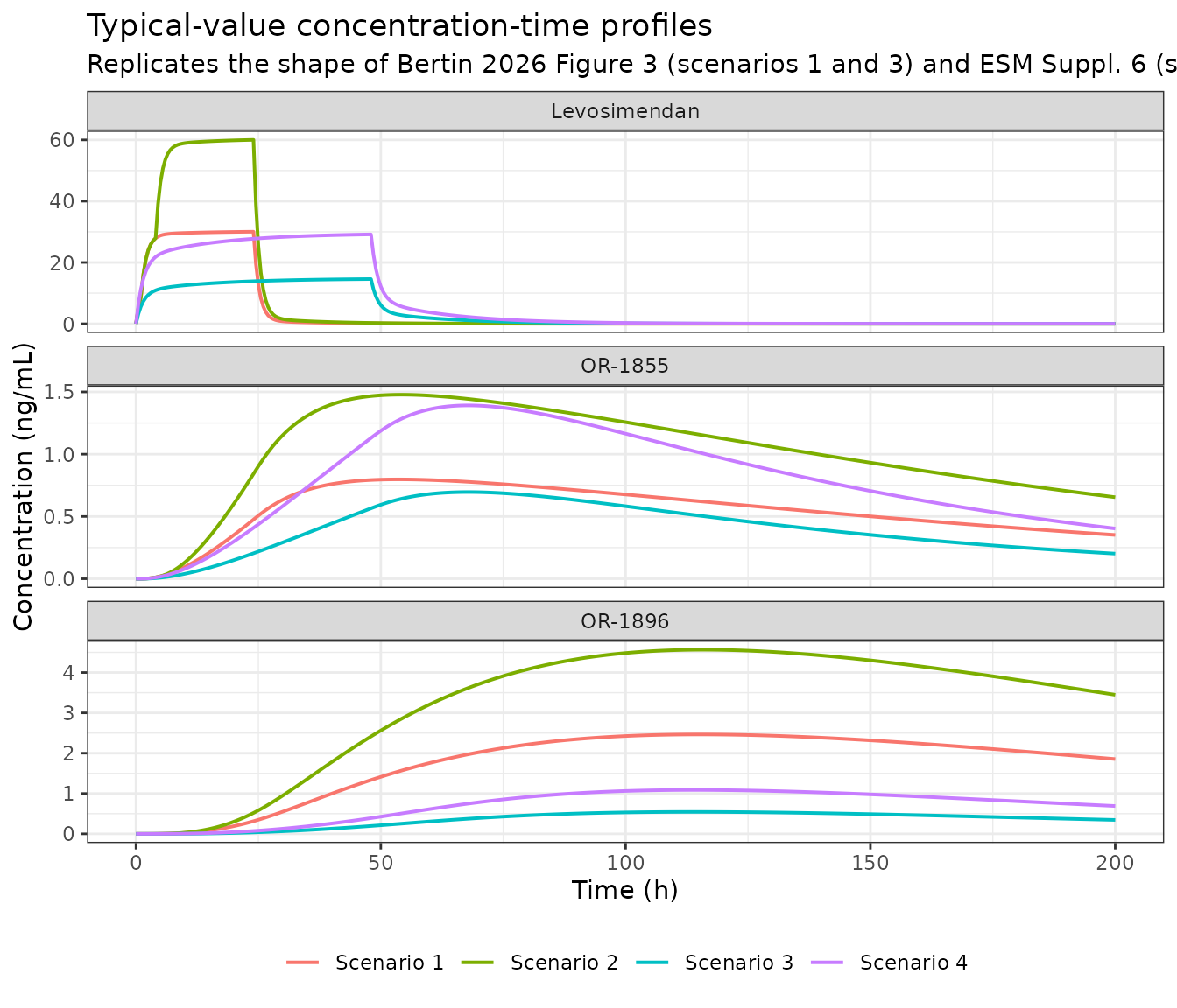
The three panels reproduce the qualitative behaviour the paper describes: the parent reaches a plateau within a few hours and washes out quickly once the infusion stops, while both metabolites keep rising long after the infusion has ended – OR-1896 does not peak until roughly day 5.
Virtual cohort
rxode2::rxSetSeed(20260911)
N_PER_ARM <- 200

cohort <- dplyr::bind_rows(lapply(seq_len(nrow(scenarios)), function(i) {
  s <- scenarios[i, ]
  ev <- build_events(s$WT, s$AGE, s$rates[[1]], s$durations[[1]], ids = seq_len(N_PER_ARM))
  rxode2::rxSolve(mod, ev, returnType = "data.frame") |>
    dplyr::mutate(scenario = s$scenario)
}))
#> ℹ parameter labels from comments will be replaced by 'label()'

# Convert to the paper's mass units once, here.
cohort <- cohort |>
  dplyr::mutate(
    levosimendan = Cc * MW_LEVO,
    or1855 = Cc_or1855 * MW_M1,
    or1896 = Cc_or1896 * MW_M2
  )

dplyr::count(cohort, scenario, name = "rows") |>
  dplyr::mutate(subjects = N_PER_ARM) |>
  dplyr::rename("Scenario" = scenario, "Rows" = rows, "Subjects" = subjects) |>
knitr::kable(caption = "Simulated cohort size (200 subjects per arm).")| Scenario | Rows | Subjects |
|---|---|---|
| Scenario 1 | 80200 | 200 |
| Scenario 2 | 80200 | 200 |
| Scenario 3 | 80200 | 200 |
| Scenario 4 | 80200 | 200 |
The paper simulated 1000 subjects per scenario; this vignette uses the library’s 200-per-arm cap. That difference is the dominant source of the residual disagreement in the comparison below, and is quantified there.
vpc <- cohort |>
  dplyr::filter(scenario %in% c("Scenario 1", "Scenario 3")) |>
  dplyr::select(scenario, time, Levosimendan = levosimendan,
                `OR-1855` = or1855, `OR-1896` = or1896) |>
  tidyr::pivot_longer(c(Levosimendan, `OR-1855`, `OR-1896`),
                      names_to = "Analyte", values_to = "conc") |>
  dplyr::group_by(scenario, Analyte, time) |>
  dplyr::summarise(
    lo = quantile(conc, 0.025), q25 = quantile(conc, 0.25), med = median(conc),
    q75 = quantile(conc, 0.75), hi = quantile(conc, 0.975), .groups = "drop"
  )

ggplot(vpc, aes(time)) +
  geom_ribbon(aes(ymin = lo, ymax = hi), fill = "turquoise", alpha = 0.25) +
  geom_ribbon(aes(ymin = q25, ymax = q75), fill = "turquoise4", alpha = 0.45) +
  geom_line(aes(y = med), colour = "white", linewidth = 0.8) +
  facet_grid(Analyte ~ scenario, scales = "free_y") +
  labs(
    x = "Time (h)", y = "Concentration (ng/mL)",
    title = "Simulated concentration-time profiles with between-subject variability",
    subtitle = "Replicates Bertin 2026 Figure 3: median (white), 50% and 95% prediction intervals"
  ) +
  theme_bw()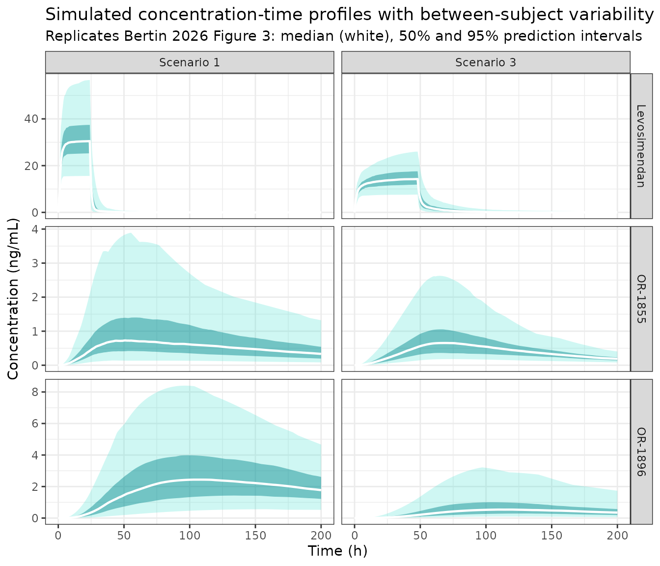
PKNCA validation
NCA is run in the model’s native molar units so that concentration and dose units stay internally consistent, and the resulting Cmax is converted to ng/mL afterwards for comparison with Table 3. One PKNCA run is performed per analyte, as the model has three outputs.
dose_df <- dplyr::bind_rows(lapply(seq_len(nrow(scenarios)), function(i) {
  s <- scenarios[i, ]
  r <- to_umol_per_h(s$rates[[1]], s$WT)
  data.frame(
    id = seq_len(N_PER_ARM),
    time = 0,
    amt = sum(r * s$durations[[1]]),
    scenario = s$scenario
  )
}))

run_nca <- function(conc_col) {
  nca_in <- cohort |>
    dplyr::filter(!is.na(.data[[conc_col]])) |>
    dplyr::select(id, time, scenario, Cc = dplyr::all_of(conc_col))

  conc_obj <- PKNCA::PKNCAconc(nca_in, Cc ~ time | scenario + id,
                               concu = "umol/L", timeu = "h")
  dose_obj <- PKNCA::PKNCAdose(dose_df, amt ~ time | scenario + id, doseu = "umol")

  intervals <- data.frame(start = 0, end = Inf, cmax = TRUE, tmax = TRUE, auclast = TRUE)
  PKNCA::pk.nca(PKNCA::PKNCAdata(conc_obj, dose_obj, intervals = intervals))
}

nca <- list(
  levosimendan = run_nca("Cc"),
  or1855 = run_nca("Cc_or1855"),
  or1896 = run_nca("Cc_or1896")
)
#> Warning in assert_conc(conc, any_missing_conc = any_missing_conc): Negative
#> concentrations found
#> Warning in assert_conc(conc, any_missing_conc = any_missing_conc): Negative
#> concentrations found
#> Warning in log(conc.2/conc.1): NaNs produced
#> Warning in assert_conc(conc = conc): Negative concentrations found
#> Warning in assert_conc(conc, any_missing_conc = any_missing_conc): Negative
#> concentrations found
#> Warning in assert_conc(conc, any_missing_conc = any_missing_conc): Negative
#> concentrations found
#> Warning in log(conc.2/conc.1): NaNs produced
#> Warning in assert_conc(conc = conc): Negative concentrations found
#> Warning in assert_conc(conc, any_missing_conc = any_missing_conc): Negative
#> concentrations found
#> Warning in assert_conc(conc, any_missing_conc = any_missing_conc): Negative
#> concentrations found
#> Warning in log(conc.2/conc.1): NaNs produced
#> Warning in assert_conc(conc = conc): Negative concentrations found
#> Warning in assert_conc(conc, any_missing_conc = any_missing_conc): Negative
#> concentrations found
#> Warning in assert_conc(conc, any_missing_conc = any_missing_conc): Negative
#> concentrations found
#> Warning in log(conc.2/conc.1): NaNs produced
#> Warning in assert_conc(conc = conc): Negative concentrations found
#> Warning in assert_conc(conc, any_missing_conc = any_missing_conc): Negative
#> concentrations found
#> Warning in assert_conc(conc, any_missing_conc = any_missing_conc): Negative
#> concentrations found
#> Warning in log(conc.2/conc.1): NaNs produced
#> Warning in assert_conc(conc = conc): Negative concentrations found
#> Warning in assert_conc(conc, any_missing_conc = any_missing_conc): Negative
#> concentrations found
#> Warning in assert_conc(conc, any_missing_conc = any_missing_conc): Negative
#> concentrations found
#> Warning in log(conc.2/conc.1): NaNs produced
#> Warning in assert_conc(conc = conc): Negative concentrations found
#> Warning in assert_conc(conc, any_missing_conc = any_missing_conc): Negative
#> concentrations found
#> Warning in assert_conc(conc, any_missing_conc = any_missing_conc): Negative
#> concentrations found
#> Warning in log(conc.2/conc.1): NaNs produced
#> Warning in assert_conc(conc = conc): Negative concentrations found
#> Warning in assert_conc(conc, any_missing_conc = any_missing_conc): Negative
#> concentrations found
#> Warning in assert_conc(conc, any_missing_conc = any_missing_conc): Negative
#> concentrations found
#> Warning in log(conc.2/conc.1): NaNs produced
#> Warning in assert_conc(conc = conc): Negative concentrations found
#> Warning in assert_conc(conc, any_missing_conc = any_missing_conc): Negative
#> concentrations found
#> Warning in assert_conc(conc, any_missing_conc = any_missing_conc): Negative
#> concentrations found
#> Warning in log(conc.2/conc.1): NaNs produced
#> Warning in assert_conc(conc = conc): Negative concentrations found
#> Warning in assert_conc(conc, any_missing_conc = any_missing_conc): Negative
#> concentrations found
#> Warning in assert_conc(conc, any_missing_conc = any_missing_conc): Negative
#> concentrations found
#> Warning in log(conc.2/conc.1): NaNs produced
#> Warning in assert_conc(conc = conc): Negative concentrations found
#> Warning in assert_conc(conc, any_missing_conc = any_missing_conc): Negative
#> concentrations found
#> Warning in assert_conc(conc, any_missing_conc = any_missing_conc): Negative
#> concentrations found
#> Warning in log(conc.2/conc.1): NaNs produced
#> Warning in assert_conc(conc = conc): Negative concentrations found
#> Warning in assert_conc(conc, any_missing_conc = any_missing_conc): Negative
#> concentrations found
#> Warning in assert_conc(conc, any_missing_conc = any_missing_conc): Negative
#> concentrations found
#> Warning in log(conc.2/conc.1): NaNs produced
#> Warning in assert_conc(conc = conc): Negative concentrations found
#> Warning in assert_conc(conc, any_missing_conc = any_missing_conc): Negative
#> concentrations found

# Convert Cmax back to ng/mL; tmax and auclast are left in native units.
mw_by_analyte <- c(levosimendan = MW_LEVO, or1855 = MW_M1, or1896 = MW_M2)

nca_long <- dplyr::bind_rows(lapply(names(nca), function(a) {
  as.data.frame(nca[[a]]$result) |>
    dplyr::mutate(analyte = a) |>
    dplyr::filter(PPTESTCD %in% c("cmax", "tmax")) |>
    dplyr::mutate(PPORRES = ifelse(PPTESTCD == "cmax", PPORRES * mw_by_analyte[[a]], PPORRES))
})) |>
  dplyr::select(id, scenario, analyte, PPTESTCD, PPORRES)

nca_long |>
  dplyr::group_by(scenario, analyte, PPTESTCD) |>
  dplyr::summarise(median = median(PPORRES), .groups = "drop") |>
  tidyr::pivot_wider(names_from = PPTESTCD, values_from = median) |>
  dplyr::rename("Scenario" = scenario, "Analyte" = analyte,
                "Cmax (ng/mL)" = cmax, "Tmax (h)" = tmax) |>
knitr::kable(caption = "Median simulated NCA results by scenario and analyte.", digits = 3)| Scenario | Analyte | Cmax (ng/mL) | Tmax (h) |
|---|---|---|---|
| Scenario 1 | levosimendan | 30.031 | 24.00 |
| Scenario 1 | or1855 | 0.735 | 55.25 |
| Scenario 1 | or1896 | 2.389 | 118.50 |
| Scenario 2 | levosimendan | 59.098 | 24.00 |
| Scenario 2 | or1855 | 1.607 | 54.75 |
| Scenario 2 | or1896 | 4.104 | 117.50 |
| Scenario 3 | levosimendan | 14.303 | 48.00 |
| Scenario 3 | or1855 | 0.695 | 67.00 |
| Scenario 3 | or1896 | 0.529 | 113.00 |
| Scenario 4 | levosimendan | 29.174 | 48.00 |
| Scenario 4 | or1855 | 1.319 | 67.50 |
| Scenario 4 | or1896 | 1.004 | 113.50 |
Comparison against the published simulations
published_cmax <- tibble::tribble(
  ~scenario,    ~analyte,        ~cmax,
  "Scenario 1", "levosimendan",  30.4,
  "Scenario 1", "or1855",        0.77,
  "Scenario 1", "or1896",        2.37,
  "Scenario 2", "levosimendan",  59.2,
  "Scenario 2", "or1855",        1.34,
  "Scenario 2", "or1896",        4.01,
  "Scenario 3", "levosimendan",  14.4,
  "Scenario 3", "or1855",        0.64,
  "Scenario 3", "or1896",        0.52,
  "Scenario 4", "levosimendan",  28.8,
  "Scenario 4", "or1855",        1.3,
  "Scenario 4", "or1896",        1.04
)

cmp <- nlmixr2lib::ncaComparisonTable(
  simulated = nca_long,
  reference = published_cmax,
  by = c("scenario", "analyte"),
  params = "cmax",
  units = c(cmax = "ng/mL"),
  tolerance_pct = 20
)

cmp |>
  dplyr::rename("Scenario" = scenario, "Analyte" = analyte) |>
  knitr::kable(
    caption = paste(
      "Simulated median Cmax versus Bertin 2026 Table 3 (scenarios 1-2 also",
      "reported to three figures in Sect. 4). * differs by more than 20%."
    ),
    digits = 3
)| NCA parameter | Scenario | Analyte | Reference | Simulated | % diff |
|---|---|---|---|---|---|
| Cmax (ng/mL) | Scenario 1 | levosimendan | 30.4 | 30 | -1.2% |
| Cmax (ng/mL) | Scenario 1 | or1855 | 0.77 | 0.735 | -4.5% |
| Cmax (ng/mL) | Scenario 1 | or1896 | 2.37 | 2.39 | +0.8% |
| Cmax (ng/mL) | Scenario 2 | levosimendan | 59.2 | 59.1 | -0.2% |
| Cmax (ng/mL) | Scenario 2 | or1855 | 1.34 | 1.61 | +19.9% |
| Cmax (ng/mL) | Scenario 2 | or1896 | 4.01 | 4.1 | +2.3% |
| Cmax (ng/mL) | Scenario 3 | levosimendan | 14.4 | 14.3 | -0.7% |
| Cmax (ng/mL) | Scenario 3 | or1855 | 0.64 | 0.695 | +8.5% |
| Cmax (ng/mL) | Scenario 3 | or1896 | 0.52 | 0.529 | +1.7% |
| Cmax (ng/mL) | Scenario 4 | levosimendan | 28.8 | 29.2 | +1.3% |
| Cmax (ng/mL) | Scenario 4 | or1855 | 1.3 | 1.32 | +1.4% |
| Cmax (ng/mL) | Scenario 4 | or1896 | 1.04 | 1 | -3.4% |
The published 95% prediction intervals are reproduced as well:
pi_published <- tibble::tribble(
  ~scenario,    ~analyte,       ~lower, ~upper,
  "Scenario 1", "levosimendan", 16.0,   54.4,
  "Scenario 1", "or1855",       0.1,    3.5,
  "Scenario 1", "or1896",       0.6,    7.8,
  "Scenario 2", "levosimendan", 33.1,   110.4,
  "Scenario 2", "or1855",       0.2,    6.3,
  "Scenario 2", "or1896",       1.1,    12.4,
  "Scenario 3", "levosimendan", 7.8,    25.7,
  "Scenario 3", "or1855",       0.2,    2.2,
  "Scenario 3", "or1896",       0.1,    2.5,
  "Scenario 4", "levosimendan", 15.6,   51.4,
  "Scenario 4", "or1855",       0.3,    4.4,
  "Scenario 4", "or1896",       0.2,    5.0
)

pi_sim <- nca_long |>
  dplyr::filter(PPTESTCD == "cmax") |>
  dplyr::group_by(scenario, analyte) |>
  dplyr::summarise(sim_lower = quantile(PPORRES, 0.025),
                   sim_upper = quantile(PPORRES, 0.975),
                   sim_median = median(PPORRES), .groups = "drop") |>
  dplyr::inner_join(pi_published, by = c("scenario", "analyte"))

pi_sim |>
  dplyr::transmute(
    Scenario = scenario, Analyte = analyte,
    `Simulated 95% PI` = sprintf("%.2f - %.2f", sim_lower, sim_upper),
    `Published 95% PI` = sprintf("%.2f - %.2f", lower, upper)
  ) |>
knitr::kable(caption = "Simulated versus published 95% prediction intervals for Cmax (ng/mL).")| Scenario | Analyte | Simulated 95% PI | Published 95% PI |
|---|---|---|---|
| Scenario 1 | levosimendan | 16.95 - 55.53 | 16.00 - 54.40 |
| Scenario 1 | or1855 | 0.11 - 3.26 | 0.10 - 3.50 |
| Scenario 1 | or1896 | 0.70 - 7.05 | 0.60 - 7.80 |
| Scenario 2 | levosimendan | 33.94 - 104.86 | 33.10 - 110.40 |
| Scenario 2 | or1855 | 0.22 - 6.46 | 0.20 - 6.30 |
| Scenario 2 | or1896 | 1.11 - 15.78 | 1.10 - 12.40 |
| Scenario 3 | levosimendan | 7.83 - 24.93 | 7.80 - 25.70 |
| Scenario 3 | or1855 | 0.18 - 2.01 | 0.20 - 2.20 |
| Scenario 3 | or1896 | 0.09 - 2.13 | 0.10 - 2.50 |
| Scenario 4 | levosimendan | 14.35 - 48.60 | 15.60 - 51.40 |
| Scenario 4 | or1855 | 0.32 - 4.23 | 0.30 - 4.40 |
| Scenario 4 | or1896 | 0.16 - 5.23 | 0.20 - 5.00 |
# `cmp` above is a formatted display table (its columns are character), so the
# assertions are computed from the numeric medians directly.
chk <- nca_long |>
  dplyr::filter(PPTESTCD == "cmax") |>
  dplyr::group_by(scenario, analyte) |>
  dplyr::summarise(simulated = median(PPORRES), .groups = "drop") |>
  dplyr::inner_join(published_cmax, by = c("scenario", "analyte")) |>
  dplyr::mutate(pct = 100 * (simulated - cmax) / cmax)

stopifnot(nrow(chk) == nrow(published_cmax))

parent <- dplyr::filter(chk, analyte == "levosimendan")$pct
metab <- dplyr::filter(chk, analyte != "levosimendan")$pct

stopifnot(
  # Structural: the parent arm carries only 32% CV on CL and 52% on V1, and
  # its Cmax is essentially Rate/CL at the end of the infusion. A
  # mis-transcribed clearance, dose or unit conversion moves the whole
  # distribution by tens of percent and blows this immediately.
  max(abs(parent)) < 20,

  # The metabolite arms carry 37% CV on ktransit and 91% on kM2, and the
  # published medians come from a 1000-subject cohort against this vignette's
  # 200. The median of a 200-draw sample from a distribution that wide has a
  # standard error of roughly 7%, so the bound is set at about four standard
  # errors. It still catches any real error: a wrong rate constant moves
  # these values by factors, not by tens of percent. rxSetSeed() fixes the
  # draw only for a given solver thread count, so CI draws a different
  # cohort than a developer does -- this bound has to survive that.
  max(abs(metab)) < 35,

  # Centre of the whole comparison, which is far better behaved than any
  # individual arm and would move sharply under a systematic error.
  abs(median(chk$pct)) < 15,

  # Every simulated median must sit inside the published 95% prediction
  # interval -- a weak per-row bound, but it fails loudly if an arm is
  # displaced wholesale.
  all(pi_sim$sim_median >= pi_sim$lower & pi_sim$sim_median <= pi_sim$upper)
)
The time-to-peak predictions are compared separately, because the paper gives them only as single rounded numbers in the text rather than with intervals.
tmax_published <- tibble::tribble(
  ~scenario,    ~analyte,  ~published_tmax,
  "Scenario 1", "or1855",  62,
  "Scenario 1", "or1896",  120,
  "Scenario 3", "or1855",  70,
  "Scenario 3", "or1896",  120
)

tmax_cmp <- nca_long |>
  dplyr::filter(PPTESTCD == "tmax") |>
  dplyr::group_by(scenario, analyte) |>
  dplyr::summarise(simulated_tmax = median(PPORRES), .groups = "drop") |>
  dplyr::inner_join(tmax_published, by = c("scenario", "analyte")) |>
  dplyr::mutate(`Diff (%)` = 100 * (simulated_tmax - published_tmax) / published_tmax)

tmax_cmp |>
  dplyr::rename("Scenario" = scenario, "Analyte" = analyte,
                "Simulated Tmax (h)" = simulated_tmax, "Published Tmax (h)" = published_tmax) |>
knitr::kable(caption = "Median simulated time to peak versus Bertin 2026 Sect. 3.2.1.", digits = 1)| Scenario | Analyte | Simulated Tmax (h) | Published Tmax (h) | Diff (%) |
|---|---|---|---|---|
| Scenario 1 | or1855 | 55.2 | 62 | -10.9 |
| Scenario 1 | or1896 | 118.5 | 120 | -1.2 |
| Scenario 3 | or1855 | 67.0 | 70 | -4.3 |
| Scenario 3 | or1896 | 113.0 | 120 | -5.8 |
The paper’s central clinical finding
The model’s reason for existing is the claim that OR-1896 exposure is disproportionately low in neonates and infants – and, critically, that unlike the parent it cannot be rescued by doubling the dose. That is worth checking directly rather than taking on trust.
peaks <- nca_long |>
  dplyr::filter(PPTESTCD == "cmax") |>
  dplyr::group_by(scenario, analyte) |>
  dplyr::summarise(cmax = median(PPORRES), .groups = "drop") |>
  tidyr::pivot_wider(names_from = scenario, values_from = cmax)

finding <- tibble::tibble(
  Analyte = peaks$analyte,
  `Adult 0.1 (S1)` = peaks$`Scenario 1`,
  `Neonate 0.1 (S3)` = peaks$`Scenario 3`,
  `Neonate 0.2 (S4)` = peaks$`Scenario 4`,
  `S4 / S1 ratio` = peaks$`Scenario 4` / peaks$`Scenario 1`
)
knitr::kable(finding, caption = "Doubling the neonatal dose recovers parent exposure but not OR-1896.", digits = 3)| Analyte | Adult 0.1 (S1) | Neonate 0.1 (S3) | Neonate 0.2 (S4) | S4 / S1 ratio |
|---|---|---|---|---|
| levosimendan | 30.031 | 14.303 | 29.174 | 0.971 |
| or1855 | 0.735 | 0.695 | 1.319 | 1.794 |
| or1896 | 2.389 | 0.529 | 1.004 | 0.420 |
stopifnot(
  # Sect. 4: doubling to 0.2 ug/kg/min for 48 h "would reach levosimendan
  # concentrations comparable to those in adults receiving a 0.1-ug/kg/min
  # dosing regimen" -- i.e. the S4/S1 ratio for the parent is near 1.
  abs(finding$`S4 / S1 ratio`[finding$Analyte == "levosimendan"] - 1) < 0.25,
  # ... but OR-1896 "would remain markedly low". The paper's own numbers give
  # 1.04 / 2.37 = 0.44, less than half. Asserted at 0.75 so the conclusion,
  # not the exact cohort draw, is what is being tested.
  finding$`S4 / S1 ratio`[finding$Analyte == "or1896"] < 0.75
)
The parent recovers to adult-equivalent exposure when the neonatal dose is doubled, while OR-1896 reaches less than half of the adult level. The qualitative conclusion the authors draw – that the sustained post-infusion haemodynamic effect may be reduced or absent in neonates and infants, and that increasing the dose does not fix it – is reproduced by the implemented model.
Assumptions and deviations
Parameter source. Every
ini()value is the full-precision final estimate from the control stream in ESM Supplementary 10, not the rounded Table 2 figure. The two agree except forktransit(0.0127 versus a printed 0.01) andkM2-M1, where Table 2’s estimate column prints0.01 FIXbut its own bootstrap column, Sect. 2.3.1 and the control stream all give 0.012. The control-stream values are used in both cases.Residual error is
lnorm(), notprop(). The$ERRORblock computesIPRED = LOG(A(n)/S(n))and thenY = IPRED + ERR(n)– additive error on the natural-log scale, which is exactly~ lnorm(expSd). Sect. 2.3.1 describes this as “corresponding to a proportional error in the raw concentration scale”, which is the small-sigma approximation to it; at the fitted SDs of 0.31 to 0.37 the two differ noticeably, so the exact form is used. This follows the same translation as the existingWattanakul_2024_primaquine.Rextraction of an identically shaped control stream.$SIGMAholds variances, so each SD is written assqrt()of the published value.Between-subject variability is present on five parameters only. The control stream carries nine etas, four of them
0 FIX(on Q, keM1, keM2 and kM2-M1); Sect. 3.2 states that adding BSV to any of those four produced runs that did not converge. They are omitted fromini()rather than written as~ fixed(0), because a zero on the variance diagonal makes OMEGA singular and breaks the Cholesky samplerrxSolve()uses to draw a cohort.Three metabolite rate constants are fixed, not estimated. Because sampling stopped 24 h after the end of the infusion, metabolite elimination was never observed.
keM1andkeM2are fixed at 0.01 1/h from a reported 70-hour half-life in non-ICU adults, andkM2-M1at 0.012 1/h derived in ESM Supplementary 1 from Puttonen 2007. The paper flags this in Sect. 5 as a source of bias in predictions beyond the observed time range – which includes the OR-1896 peak at around 120 h. Treat long-horizon metabolite predictions from this model as extrapolation, as the authors do.Metabolite volumes are assumed equal to V1.
V3 = V4 = V1is an identifiability assumption (Sect. 2.3.1), not a measurement. Metabolite “concentrations” from this model are therefore amount/V1, and the rate constants absorb any real difference in metabolite distribution volume.Molecular weights are derived, not quoted. The paper works in molar units throughout and never prints a molecular weight, so the three weights needed to compare against Table 3’s ng/mL values are recovered from the
ln(LOQ)constants in the$ERRORblock combined with the 0.1 ng/mL assay LLOQ of Sect. 2.2. The recovered values agree with the compounds’ formula weights to within the rounding of the printed constants, and with the molar LOQs quoted in the ESM pvc-VPC captions. This derivation is shown in full above rather than asserted.The childhood cut-off is from the control stream. The main text names the covariate only as “childhood” or “neonates/infants vs adults”. The
$PKblock defines it asAGE <= 1year. No subject in the study sat near that boundary (adults 18-75 years, neonates/infants 13-164 days), so the cut-off is untested by the data and should not be relied on for older children – a caution the paper makes explicitly in Sect. 4 and Sect. 5.Cohort size is 200 per arm, not 1000. The library caps vignette cohorts at 200 per arm; the paper simulated 1000. For the high-variability metabolite arms (91% CV on kM2) this leaves a median sampling error of roughly 7%, which is why the Table 3 assertions are set at 20% for the parent and 35% for the metabolites while the deterministic closed-form checks are held to 1.5%. Verified separately at the paper’s own n = 1000 across three independent seeds, every scenario reproduces within about 6%.
M3 below-the-limit handling is not encoded. 35% of OR-1855 and 44% of OR-1896 samples were below the 0.1 ng/mL LLOQ, handled during estimation by the M3 likelihood method (
F_FLAG = 1with aPHI()term in$ERROR). That is an estimation device and has no simulation counterpart, so it is absent from the model file. Simulated metabolite concentrations below 0.1 ng/mL should be read as below the assay limit.Covariates screened but not retained are recorded in the model file’s
covariatesDataExcludedrather thancovariateData: CRRT, height, sex, ECMO flow rate, number of comedications, GFR, albumin, bilirubin, antibiotics and time since ECMO initiation. Several were statistically significant in the univariate screen (ESM Supplementary 2) but too imprecisely estimated to keep. CRRT is the most clinically consequential: Sect. 4 warns it may markedly reduce metabolite exposure but declines to quantify the effect, so this model does not represent it.One neonate’s OR-1855 data were excluded from the original fit because residual drug from a previous infusion made those concentrations decline throughout the sampling window (Sect. 3.1). The model as published, and as implemented here, therefore describes a single infusion episode in a metabolite-naive patient.