Alprazolam (Klein 2026)
Source:vignettes/articles/Klein_2026_alprazolam.Rmd
Klein_2026_alprazolam.RmdModel and source
#> ℹ parameter labels from comments will be replaced by 'label()'Citation: Klein P, Aungaroon G, Biton V, Liow KK, Phillips S, Wychowski T, Sadek A, Elshoff JP, Roebling R, King A, Rospo CC, Schoemaker R, Chanteux H. Pharmacokinetics and tolerability of single-dose Staccato alprazolam in adolescents with epilepsy, and population pharmacokinetic analysis to support dose selection in adolescents. Epilepsia. 2026;67(1):109-119. doi:10.1111/epi.18643. Population PK parameters are from Supporting Information Table S3.
Description: Two-compartment population pharmacokinetic model for inhaled alprazolam delivered by the Staccato(R) hand-held thermal-aerosol device, pooled across three trials in adults and adolescents with epilepsy (Klein 2026, N = 99). Absorption is modelled as two parallel processes whose fractions sum to 1: an immediate-release fraction that enters the central compartment as a bolus at the dose time (the paper’s F2 = 0.369 ‘fast absorption fraction’), and the complementary fraction that enters a depot compartment and is absorbed first-order with ka = 5.37 /h (absorption half-life 7.74 min). Both fractions are supplied from the same administered dose, so an event table must carry TWO dose records at each administration time, one to depot and one to central; the f() terms then split the dose. The dose fraction is carried on the logit scale (the library’s logitfdepot idiom) so individual values stay inside (0, 1) – the paper’s own 95% CI for F2 is exactly symmetric on the logit scale, which proves the authors estimated it there. All disposition parameters are apparent (/F): the inhaled bioavailability is not separately identifiable. No relationship between body weight and clearance or intercompartmental clearance was detectable, so allometric scaling is applied only to the central and peripheral volumes, through a single freely estimated exponent shared by both. Clearance carries a multiplicative increase with concomitant strong hepatic enzyme-inducing antiseizure medications (carbamazepine, phenobarbital, phenytoin, or primidone). Interindividual variability is log-normal on ka, CL, Vc, Q and Vp (with CL and Vc correlated) and normal on the logit dose fraction; residual error is proportional.
Article: https://doi.org/10.1111/epi.18643
Supporting Information (Tables S1-S3, Figures S1-S5): distributed with the open-access article (PMC12893244).
Staccato alprazolam is a hand-held, breath-actuated thermal-aerosol device that vaporises alprazolam and delivers it to the deep lung, where it is absorbed at the alveolar-capillary interface. The population PK model reported here pools adolescent data from the Phase 1 trial UP0100 with adult data from two earlier trials, and was used to support the 2 mg adolescent dose in the Phase 3 programme.
Population
| Field | Value |
|---|---|
| species | human |
| n_subjects | 99 |
| n_studies | 3 |
| age_range | 12-17 years (adolescents, UP0100); adults in AMDC-002-202 and ENGAGE-E-001 |
| age_median | 32.2 years (mean, SD 13.5) overall; 15.1 years (mean, SD 1.90) in the adolescent trial |
| weight_range | 33.5-81.2 kg in the adolescent trial UP0100; overall mean 75.5 kg (SD 22.5) |
| weight_median | 75.5 kg (mean) overall; 54.4 kg (mean) in the adolescent trial |
| sex_female_pct | 70.7 |
| race_ethnicity | White: 78.6; Pacific Islander: 7.1; Other/mixed: 14.3 |
| disease_state | focal, generalized, or focal and generalized epilepsy; photosensitive epilepsy in AMDC-002-202 |
| dose_range | single inhaled dose of Staccato alprazolam 0.5, 1 or 2 mg |
| regions | United States (UP0100); regions not reported for AMDC-002-202 or ENGAGE-E-001 |
| co_medication | 15/99 (15.2%) on a strong enzyme-inducing antiseizure medication; 27/99 (27.3%) chronic benzodiazepine users |
| notes | Pooled analysis dataset of three trials (Table S1): UP0100 (Phase 1, adolescents, N = 14, NCT04857307), AMDC-002-202 (Phase 2a, adults with photosensitive epilepsy, N = 5, NCT02351115) and ENGAGE-E-001 (Phase 2b, adults with epilepsy, N = 80, NCT03478982). Race percentages are from the adolescent trial only (Table S2); race is not reported for the pooled dataset. The main text reports N = 84 enrolled in ENGAGE-E-001 while Table S1 reports N = 80 in the PK modelling dataset. |
The analysis dataset (Table S1) pools 99 subjects from 3 trials: UP0100 (Phase 1, 14 adolescents aged 12-17 years with focal, generalized, or focal and generalized epilepsy, NCT04857307), AMDC-002-202 (Phase 2a, 5 adults with photosensitive epilepsy, NCT02351115) and ENGAGE-E-001 (Phase 2b, 80 adults with epilepsy, NCT03478982). Overall mean age was 32.2 years (SD 13.5) and mean weight 75.5 kg (SD 22.5); 70.7% were female. Fifteen subjects (15.2%), all in ENGAGE-E-001, were taking a strong hepatic enzyme-inducing antiseizure medication; no adolescent was, because UP0100 excluded patients on strong CYP3A4 inducers by protocol.
Model structure
Absorption is modelled as two parallel processes whose fractions sum to one:
- an immediate-release fraction that appears in
centralas a bolus at the dose time (the paper’sF2= 0.369, the “fast absorption fraction”), and - the complementary fraction (0.631) that enters
depotand is absorbed first-order withka= 5.37 /h, i.e. an absorption half-life of 7.74 min.
Because both arms are fed from the same administered dose,
an event table for this model must carry two dose records at
each administration time – one to depot and one to
central. The f(depot) /
f(central) terms then apportion them. Every cohort below
follows that pattern.
Disposition is two-compartment with linear elimination. Body weight scales the central and peripheral volumes through a single shared exponent; it does not scale CL or Q, because the authors could detect no weight relationship for either (Methods section 2.2, and the title of Table S3).
Source trace
Every value below is also carried as an in-file comment beside its
ini() entry in
inst/modeldb/specificDrugs/Klein_2026_alprazolam.R.
| Equation / parameter | Value | Source location |
|---|---|---|
lka |
5.37 /h (95% CI 3.88-7.45) | Table S3, row ka; absorption half-life 7.74 (5.58-10.7)
min restated in Results section 3.2 |
lcl |
8.23 L/h (7.23-9.38) | Table S3, row CL/F; restated in Results section
3.2 |
lvc |
36.9 L (23.1-59.2) | Table S3, row Vc/F
|
lq |
189 L/h (131-271) | Table S3, row Q/F
|
lvp |
60.3 L (47.2-77.0) | Table S3, row Vp/F
|
logitfdepot |
qlogis(1 - 0.369) |
Table S3, row F2 = 0.369 (0.156-0.649); restated in
Results section 3.2 |
e_wt_vc_vp |
0.470 (0.341-0.598) | Table S3, row Allometric scaling Vc and Vp
|
e_conmed_eiaed_cl |
log(1.955) |
Table S3, row Effect of inducer ASMs on CL, % change =
95.5 (50.5-154.0) |
etalka |
0.730^2 | Table S3, IIV column, row ka = 73.0% |
etalcl, etalvc block |
0.586^2, 0.763^2, r = 0.342 | Table S3, IIV column rows CL/F 58.6% and
Vc/F 76.3%; footnote “Correlation between CL and Vc:
0.342” |
etalq |
0.396^2 | Table S3, IIV column, row Q/F = 39.6% |
etalvp |
0.209^2 | Table S3, IIV column, row Vp/F = 20.9% |
etalogitfdepot |
1.078^2 | Table S3, IIV column, row F2 = 107.8% |
propSd |
0.100 | Table S3, row Proportional RUV, % = 10.0
(8.30-11.7) |
| Two parallel absorption arms; 2-compartment disposition; linear elimination | n/a | Methods section 2.2, paragraph 3 |
| No weight effect on CL or Q; shared allometric exponent on Vc and Vp | n/a | Methods section 2.2, paragraph 4, and Table S3 title |
WT reference 70 kg |
assumed | not stated in the paper; see Assumptions below |
How each estimation scale was identified
Table S3 reports a 95% CI for every structural parameter but never states the scale each was estimated on. Each CI is Wald-symmetric on exactly one scale, so the CIs identify the scales without any appeal to convention. Recomputing the midpoint on each candidate scale and comparing with the published point estimate:
ci <- tibble::tribble(
  ~parameter,  ~estimate, ~lower,  ~upper,
  "ka",             5.37,   3.88,    7.45,
  "CL/F",           8.23,   7.23,    9.38,
  "Vc/F",          36.9,   23.1,    59.2,
  "Q/F",          189,    131,     271,
  "Vp/F",          60.3,   47.2,    77.0,
  "F2",             0.369,  0.156,   0.649,
  "Allom. exp.",    0.470,  0.341,   0.598,
  "Prop. RUV (%)", 10.0,    8.30,   11.7
)

# The logit scale is only defined for a bound in (0, 1); return NA elsewhere
# rather than letting qlogis() emit NaN.
logit_mid <- function(lower, upper) {
  ok <- lower > 0 & lower < 1 & upper > 0 & upper < 1
  ifelse(ok, plogis((qlogis(ifelse(ok, lower, 0.5)) +
                       qlogis(ifelse(ok, upper, 0.5))) / 2), NA_real_)
}

scale_check <- ci |>
  mutate(
    linear = (lower + upper) / 2,
    log    = exp((log(lower) + log(upper)) / 2),
    logit  = logit_mid(lower, upper),
    err    = pmin(abs(linear / estimate - 1),
                  abs(log / estimate - 1),
                  abs(logit / estimate - 1), na.rm = TRUE),
    best   = c("linear", "log", "logit")[
      apply(cbind(abs(linear / estimate - 1),
                  abs(log / estimate - 1),
                  abs(logit / estimate - 1)), 1,
            \(x) which.min(replace(x, is.na(x), Inf)))]
  )

scale_check |>
  mutate(across(c(linear, log, logit), \(x) signif(x, 4))) |>
  dplyr::rename("Parameter" = parameter, "Published estimate" = estimate,
                "Midpoint, linear" = linear, "Midpoint, log" = log,
                "Midpoint, logit" = logit, "Scale identified" = best) |>
  dplyr::select(-lower, -upper, -err) |>
knitr::kable(caption = "CI midpoint on each candidate scale vs the published point estimate. The scale whose midpoint reproduces the estimate is the scale the parameter was estimated on.")| Parameter | Published estimate | Midpoint, linear | Midpoint, log | Midpoint, logit | Scale identified |
|---|---|---|---|---|---|
| ka | 5.370 | 5.6650 | 5.3760 | NA | log |
| CL/F | 8.230 | 8.3050 | 8.2350 | NA | log |
| Vc/F | 36.900 | 41.1500 | 36.9800 | NA | log |
| Q/F | 189.000 | 201.0000 | 188.4000 | NA | log |
| Vp/F | 60.300 | 62.1000 | 60.2900 | NA | log |
| F2 | 0.369 | 0.4025 | 0.3182 | 0.3689 | logit |
| Allom. exp. | 0.470 | 0.4695 | 0.4516 | 0.4673 | linear |
| Prop. RUV (%) | 10.000 | 10.0000 | 9.8540 | NA | linear |
F2 is only interpretable on the logit
scale: its logit midpoint reproduces 0.369 to three decimals, while the
linear midpoint gives 0.4025 and the log midpoint 0.3182. That is
decisive, and it is corroborated structurally – a log-normal IIV of the
reported magnitude on a fraction bounded by 1 would push roughly 13% of
subjects above F2 = 1, i.e. a negative depot fraction. The
model therefore carries the dose fraction on the logit scale, using the
library’s logitfdepot idiom.
The inducer effect is likewise a log-scale coefficient: the midpoint
of log(1.505) and log(2.540) is 0.67048, which
is log(1.955) to five decimals, whereas the linear midpoint
of the reported percentages is 102.25%, not 95.5%.
# Every parameter's estimation scale must be recovered from its own CI.
stopifnot(identical(
  scale_check$best,
  c("log", "log", "log", "log", "log", "logit", "linear", "linear")
))
# ...and on that scale the midpoint must reproduce the estimate to within 0.5%.
stopifnot(!anyNA(scale_check$err), all(scale_check$err < 0.005))
Which reading of the “IIV” column?
Table S3 reports interindividual variability as a bare percentage with no back-transformation stated. Two readings are current in the literature and they differ by about 8% on omega:
- omega is the standard deviation on the parameter’s
own estimation scale, reported as
omega * 100– for CL that gives omega = 0.586; - the percentage is the exact log-normal CV%,
sqrt(exp(omega^2) - 1) * 100– for CL that gives omega = 0.543.
Figure 4 settles it in closed form, with no simulation and no
digitising of a curve. The Supplementary Methods state that AUCinf was
computed “using the sampled clearance (CL) parameter by dividing the
administered dose by CL”, so the simulated AUCinf distribution is
exactly log-normal with median dose / CL and 5th/95th
percentiles median * exp(-/+ 1.645 * omega_CL). Only one
reading can match the published band.
dose_ug   <- 2000          # 2 mg expressed in ug so AUC comes out in ng*h/mL
cl_typ    <- 8.23
inducer   <- 1.955         # CL multiplier with an enzyme-inducing ASM

omega_sd  <- 0.586                          # "IIV % is omega * 100"
omega_cv  <- sqrt(log(1 + 0.586^2))         # "IIV % is the exact log-normal CV%"

band <- function(omega, cl) {
  med <- dose_ug / cl
  c(p05 = med / exp(1.645 * omega), median = med, p95 = med * exp(1.645 * omega))
}

# Values read off Figure 4 (blue band and red median line, adolescent panels).
digitised <- tibble::tribble(
  ~panel,          ~p05, ~median, ~p95,
  "No inducer ASM",  93,     240,  645,
  "Inducer ASM",     45,     122,  330
)

iiv_cmp <- bind_rows(
  tibble::tibble(panel = "No inducer ASM", reading = "omega = SD (0.586)",
                 !!!band(omega_sd, cl_typ)),
  tibble::tibble(panel = "No inducer ASM", reading = "omega = exact CV% (0.543)",
                 !!!band(omega_cv, cl_typ)),
  tibble::tibble(panel = "Inducer ASM", reading = "omega = SD (0.586)",
                 !!!band(omega_sd, cl_typ * inducer)),
  tibble::tibble(panel = "Inducer ASM", reading = "omega = exact CV% (0.543)",
                 !!!band(omega_cv, cl_typ * inducer))
) |>
  left_join(digitised, by = "panel", suffix = c("", "_fig")) |>
  mutate(`error, 5th (%)`  = 100 * (p05 / p05_fig - 1),
         `error, 95th (%)` = 100 * (p95 / p95_fig - 1))

iiv_cmp |>
  mutate(across(where(is.numeric), \(x) round(x, 1))) |>
  dplyr::select(panel, reading, p05, p95, p05_fig, p95_fig,
                `error, 5th (%)`, `error, 95th (%)`) |>
  dplyr::rename("Figure 4 panel" = panel, "Reading of the IIV column" = reading,
                "5th, predicted" = p05, "95th, predicted" = p95,
                "5th, Figure 4" = p05_fig, "95th, Figure 4" = p95_fig) |>
knitr::kable(caption = "AUCinf (ng*h/mL) 90% range under each reading of Table S3's IIV column, against values read off Figure 4.")| Figure 4 panel | Reading of the IIV column | 5th, predicted | 95th, predicted | 5th, Figure 4 | 95th, Figure 4 | error, 5th (%) | error, 95th (%) |
|---|---|---|---|---|---|---|---|
| No inducer ASM | omega = SD (0.586) | 92.7 | 637.2 | 93 | 645 | -0.3 | -1.2 |
| No inducer ASM | omega = exact CV% (0.543) | 99.4 | 594.0 | 93 | 645 | 6.9 | -7.9 |
| Inducer ASM | omega = SD (0.586) | 47.4 | 325.9 | 45 | 330 | 5.3 | -1.2 |
| Inducer ASM | omega = exact CV% (0.543) | 50.9 | 303.8 | 45 | 330 | 13.0 | -7.9 |
err <- iiv_cmp |>
  group_by(reading) |>
  summarise(mean_abs_err = mean(abs(c(`error, 5th (%)`, `error, 95th (%)`))),
            .groups = "drop")
# The SD reading must win, and by a clear margin, on the pooled tail error.
stopifnot(
  err$mean_abs_err[err$reading == "omega = SD (0.586)"] <
    err$mean_abs_err[err$reading == "omega = exact CV% (0.543)"],
  err$mean_abs_err[err$reading == "omega = SD (0.586)"] < 5
)
# The median is common to both readings and must land on the published line.
stopifnot(abs(dose_ug / cl_typ / 240 - 1) < 0.05,
          abs(dose_ug / (cl_typ * inducer) / 122 - 1) < 0.05)
The SD reading reproduces both tails of both panels to within a few
percent; the exact-CV% reading is systematically too narrow, missing the
no-inducer 95th percentile by about 8%. The model therefore encodes
omega = IIV% / 100 on each parameter’s own estimation
scale. The two readings differ by less than the width of the published
CIs for the structural parameters, so this choice matters for simulated
variability, not for typical-value predictions.
Structural identity checks
These four checks are deterministic: they compare the solved model against closed forms implied by the published parameters, with the random effects zeroed. They contain no cohort sampling, so they can be asserted tightly.
mod     <- readModelDb("Klein_2026_alprazolam")
mod_typ <- rxode2::zeroRe(mod)
#> ℹ parameter labels from comments will be replaced by 'label()'

# Two dose records per administration: the immediate-release arm and the depot arm.
dose_rows <- function(id, wt, eiaed) {
  tibble::tibble(id = id, WT = wt, CONMED_EIAED = eiaed, time = 0,
                 amt = 2, evid = 1L, cmt = c("depot", "central"))
}
obs_rows <- function(id, wt, eiaed, times) {
  tibble::tibble(id = id, WT = wt, CONMED_EIAED = eiaed, time = times,
                 amt = NA_real_, evid = 0L, cmt = "central")
}

wt_bands <- c(`<50 kg` = 41.27, `>=50 kg` = 64.35, `All patients` = 54.46)
grid     <- seq(0, 36, length.out = 20001)

ev_typ <- bind_rows(lapply(seq_along(wt_bands), function(i) {
  bind_rows(dose_rows(i, wt_bands[[i]], 0), obs_rows(i, wt_bands[[i]], 0, grid))
})) |> arrange(id, time, desc(evid))

sim_typ <- rxode2::rxSolve(mod_typ, ev_typ, omega = NA, sigma = NA,
                           keep = c("WT")) |> as.data.frame()
stopifnot(nrow(sim_typ) > 0, all(sim_typ$Cc >= 0))

terminal_slope <- function(d) {
  -coef(stats::lm(log(Cc) ~ time, data = d[d$time >= 12, ]))[[2]]
}
auc_inf <- function(d) {
  a <- sum(diff(d$time) * (head(d$Cc, -1) + tail(d$Cc, -1)) / 2)
  a + tail(d$Cc, 1) / terminal_slope(d)
}

published_t12 <- c(`<50 kg` = 6.816, `>=50 kg` = 8.477, `All patients` = 7.601)

ident <- lapply(seq_along(wt_bands), function(i) {
  d  <- sim_typ[sim_typ$id == i, ]
  vc <- 36.9 * (wt_bands[[i]] / 70)^0.470
  tibble::tibble(
    band            = names(wt_bands)[i],
    WT              = wt_bands[[i]],
    t12_model       = log(2) / terminal_slope(d),
    t12_published   = published_t12[[i]],
    c0_solved       = d$Cc[1],
    c0_closed_form  = 0.369 * 2 / vc * 1000,
    aucinf_solved   = auc_inf(d),
    aucinf_dose_cl  = dose_ug / cl_typ
  )
}) |> bind_rows() |>
  mutate(`t1/2 error (%)` = 100 * (t12_model / t12_published - 1),
         `C(0+) ratio`    = c0_solved / c0_closed_form,
         `AUCinf ratio`   = aucinf_solved / aucinf_dose_cl)

ident |>
  mutate(across(where(is.numeric), \(x) signif(x, 6))) |>
  dplyr::select(band, WT, t12_model, t12_published, `t1/2 error (%)`,
                `C(0+) ratio`, `AUCinf ratio`) |>
  dplyr::rename("Weight band" = band, "WT (kg)" = WT,
                "t1/2, model (h)" = t12_model,
                "t1/2, Table 1 (h)" = t12_published) |>
knitr::kable(caption = "Deterministic structural checks against closed forms and against the observed terminal half-lives in Table 1.")| Weight band | WT (kg) | t1/2, model (h) | t1/2, Table 1 (h) | t1/2 error (%) | C(0+) ratio | AUCinf ratio |
|---|---|---|---|---|---|---|
| <50 kg | 41.27 | 6.49434 | 6.816 | -4.71923 | 1 | 1 |
| >=50 kg | 64.35 | 8.00211 | 8.477 | -5.60212 | 1 | 1 |
| All patients | 54.46 | 7.39849 | 7.601 | -2.66425 | 1 | 1 |
# 1. The immediate-release bolus must be exactly F2 * dose / Vc(WT).
stopifnot(max(abs(ident$`C(0+) ratio` - 1)) < 1e-6)

# 2. AUCinf must be exactly dose / CL, and independent of weight, because the
#    paper found no weight effect on CL.
#    (relative tolerances: the comparator is a trapezoidal integral, so the
#    residual is numerical-quadrature error, not model error)
stopifnot(max(abs(ident$`AUCinf ratio` - 1)) < 1e-4,
          diff(range(ident$aucinf_solved)) / mean(ident$aucinf_solved) < 1e-4)

# 3. The model's terminal half-lives must reproduce the observed ones in Table 1,
#    including the ORDERING across weight bands -- that ordering is generated
#    purely by the allometric exponent on Vc and Vp, since CL is not scaled.
stopifnot(max(abs(ident$`t1/2 error (%)`)) < 10)
stopifnot(ident$t12_model[ident$band == "<50 kg"] <
            ident$t12_model[ident$band == ">=50 kg"])

# 4. The enzyme-inducer effect must divide exposure by exactly 1.955.
ev_ind <- bind_rows(dose_rows(1L, 70, 1), obs_rows(1L, 70, 1, grid)) |>
  arrange(time, desc(evid))
ev_non <- bind_rows(dose_rows(1L, 70, 0), obs_rows(1L, 70, 0, grid)) |>
  arrange(time, desc(evid))
auc_ind <- auc_inf(as.data.frame(rxode2::rxSolve(mod_typ, ev_ind, omega = NA, sigma = NA)))
auc_non <- auc_inf(as.data.frame(rxode2::rxSolve(mod_typ, ev_non, omega = NA, sigma = NA)))
stopifnot(abs((auc_non / auc_ind) / 1.955 - 1) < 1e-4)
The half-life check is the strongest single piece of evidence for the
assumed 70 kg reference weight. CL is not weight-scaled, so
the only thing that can make terminal half-life vary with body
weight in this model is the shared allometric exponent on
Vc and Vp. The model reproduces both the
direction and the magnitude of the observed difference between the two
adolescent weight bands (Table 1: 6.816 h below 50 kg vs 8.477 h at or
above 50 kg) without any parameter having been fitted to those
numbers.
Virtual adolescent cohort
The cohort reproduces the UP0100 demographics (Table S2): 200 adolescents with body weight drawn from a normal distribution with the observed mean 54.46 kg and SD 14.43 kg, truncated to the observed range 33.5-81.2 kg. None receives an enzyme-inducing antiseizure medication, matching the trial’s exclusion criterion. Samples are taken at the protocol times – pre-dose and 2, 10 and 30 min and 1, 2, 6, 24 and 36 h post-dose – because Cmax and Tmax in Table 1 are discrete statistics limited by that schedule, a limitation the authors call out explicitly in the Discussion.
set.seed(20260828)
n_adol <- 200

wt <- rnorm(n_adol, 54.46, 14.43)
wt <- pmin(pmax(wt, 33.5), 81.2)

subj <- tibble::tibble(
  id           = seq_len(n_adol),
  WT           = wt,
  wtgrp        = ifelse(wt < 50, "<50 kg", ">=50 kg"),
  CONMED_EIAED = 0
)

protocol_times <- c(0, 2 / 60, 10 / 60, 0.5, 1, 2, 6, 24, 36)

events <- bind_rows(
  subj |> mutate(time = 0, amt = 2, evid = 1L, cmt = "depot"),
  subj |> mutate(time = 0, amt = 2, evid = 1L, cmt = "central"),
  tidyr::crossing(subj, time = protocol_times) |>
    mutate(amt = NA_real_, evid = 0L, cmt = "central")
) |>
  arrange(id, time, desc(evid))

# The two dose records at t = 0 must be distinguished by their target
# compartment, and the t = 0 observation by its evid. Check the events
# themselves -- unique()-ing first would make this assertion unfalsifiable.
stopifnot(
  anyDuplicated(events[, c("id", "time", "evid", "cmt")]) == 0L,
  # every subject carries exactly two dose records: one per absorption arm
  nrow(dplyr::filter(events, evid == 1L)) == 2L * n_adol
)
sim <- rxode2::rxSolve(mod, events, keep = c("WT", "wtgrp")) |> as.data.frame()
#> ℹ parameter labels from comments will be replaced by 'label()'
stopifnot(nrow(sim) > 0, dplyr::n_distinct(sim$id) == n_adol)
sim carries the observation with residual error and
Cc the individual prediction; the NCA below uses
sim, because the published noncompartmental analysis was
run on measured concentrations, which carry the same 10% proportional
error.
Replicate Figure 1
LLOQ <- 0.200

gm <- function(x) {
  x <- x[is.finite(x) & x > 0]
  if (!length(x)) return(NA_real_)
  exp(mean(log(x)))
}

sim |>
  filter(time > 0) |>
  group_by(wtgrp, time) |>
  summarise(geomean = gm(sim), .groups = "drop") |>
  ggplot(aes(time, geomean, colour = wtgrp, shape = wtgrp)) +
  geom_line() + geom_point() +
  geom_hline(yintercept = LLOQ, linetype = "dashed", linewidth = 0.3) +
  scale_y_log10() +
  scale_x_continuous(breaks = seq(0, 36, by = 6)) +
  labs(x = "Time (hours)", y = "Geometric mean concentration (ng/mL)",
       colour = "Body weight", shape = "Body weight",
       title = "Figure 1 (semilogarithmic) -- simulated adolescent cohort",
       caption = "Replicates Figure 1B of Klein 2026. Dashed line: LLOQ 0.200 ng/mL.")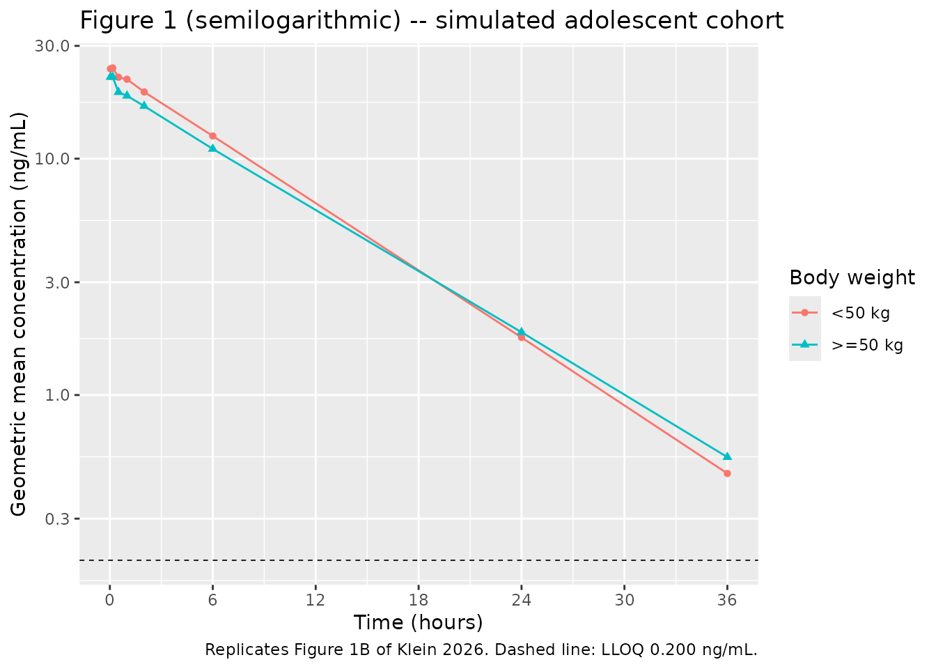
Replicates Figure 1 of Klein 2026: geometric mean plasma alprazolam concentration-time profiles by adolescent body weight group after a single 2 mg dose.
As in the published figure, the lower weight band runs above the higher one over the absorption and early distribution phases and crosses below it during the terminal phase, the latter because only the volumes – not clearance – scale with body weight.
PKNCA validation
Concentrations below the 0.200 ng/mL lower limit of quantification
are censored, so auclast is computed to the last
quantifiable concentration exactly as the published
AUC0-t was.
The immediate-release arm puts drug in central at the
instant of dosing, so the model’s time = 0 observation is a
post-bolus concentration. The trial’s pre-dose sample was taken
before administration, in drug-naive patients, and was therefore zero.
The pre-dose record is set to zero here to match, which also keeps
Cmax and Tmax derived from post-dose samples
only, exactly as in the trial.
post_dose <- sim |>
  dplyr::filter(time > 0) |>
  dplyr::select(id, time, wtgrp, Cc = sim) |>
  mutate(Cc = ifelse(Cc < LLOQ, NA_real_, Cc)) |>
  dplyr::filter(!is.na(Cc))

pre_dose <- subj |> transmute(id, wtgrp, time = 0, Cc = 0)

conc_df <- bind_rows(pre_dose, post_dose) |> arrange(id, time)

stopifnot(
  nrow(conc_df) > 0,
  # every subject must carry exactly one time-zero anchor record
  nrow(dplyr::filter(conc_df, time == 0)) == n_adol
)

dose_df <- subj |> transmute(id, wtgrp, time = 0, amt = 2)

conc_obj <- PKNCA::PKNCAconc(as.data.frame(conc_df), Cc ~ time | wtgrp + id)
dose_obj <- PKNCA::PKNCAdose(as.data.frame(dose_df), amt ~ time | wtgrp + id)

intervals <- data.frame(
  start = 0, end = Inf,
  cmax = TRUE, tmax = TRUE, auclast = TRUE, aucinf.obs = TRUE,
  half.life = TRUE, cl.obs = TRUE, vss.obs = TRUE
)

nca_res <- suppressWarnings(
  PKNCA::pk.nca(PKNCA::PKNCAdata(conc_obj, dose_obj, intervals = intervals))
)
nca_df <- as.data.frame(nca_res)
stopifnot(nrow(nca_df) > 0)
PKNCA reports cl.obs and
vss.obs in dose units per concentration unit – here mg per
(ng/mL), i.e. 1000 L – so both are rescaled to litres below before
comparison with the published CL/F and
Vss/F.
nca_scaled <- nca_df |>
  mutate(PPORRES = ifelse(PPTESTCD %in% c("cl.obs", "vss.obs"),
                          PPORRES * 1000, PPORRES),
         PPORRES = ifelse(PPTESTCD == "tmax", PPORRES * 60, PPORRES))
Comparison against published NCA
Table 1 of the paper reports geometric means for
every parameter except Tmax, which is a median.
ncaComparisonTable() aggregates a per-subject input with
median(), so the simulated results are pre-aggregated here
with the matching statistic – geometric mean throughout, median for
Tmax – and the already-summarised frame is passed in.
Comparing a simulated median against a published geometric mean would
score the two sides on different quantities.
published <- tibble::tribble(
  ~wtgrp,     ~cmax, ~aucinf.obs, ~auclast, ~cl.obs, ~tmax, ~vss.obs, ~half.life,
  "<50 kg",   38.27,       281.1,    270.8,   7.114,  19.50,    67.53,      6.816,
  ">=50 kg",  33.55,       278.8,    283.8,   7.174,  10.00,    87.38,      8.477
)

nca_summary <- nca_scaled |>
  group_by(wtgrp, PPTESTCD) |>
  summarise(PPORRES = if (first(PPTESTCD) == "tmax") {
              median(PPORRES, na.rm = TRUE)
            } else {
              gm(PPORRES)
            }, .groups = "drop")
stopifnot(nrow(nca_summary) > 0, !anyNA(nca_summary$PPORRES))

cmp <- nlmixr2lib::ncaComparisonTable(
  simulated     = as.data.frame(nca_summary),
  reference     = published,
  by            = "wtgrp",
  units         = c(cmax = "ng/mL", aucinf.obs = "ng*h/mL", auclast = "ng*h/mL",
                    cl.obs = "L/h", tmax = "min", vss.obs = "L", half.life = "h"),
  tolerance_pct = 20
)

knitr::kable(
  cmp,
  caption = "Simulated (200 virtual adolescents per weight band) vs published Table 1 of Klein 2026. * marks a difference of more than 20%."
)| NCA parameter | wtgrp | Reference | Simulated | % diff |
|---|---|---|---|---|
| Cmax (ng/mL) | <50 kg | 38.3 | 30.8 | -19.6% |
| Cmax (ng/mL) | >=50 kg | 33.6 | 27.7 | -17.4% |
| Tmax (min) | <50 kg | 19.5 | 10 | -48.7%* |
| Tmax (min) | >=50 kg | 10 | 10 | +0.0% |
| AUC0-∞ (obs) (ng*h/mL) | <50 kg | 281 | 253 | -10.1% |
| AUC0-∞ (obs) (ng*h/mL) | >=50 kg | 279 | 244 | -12.6% |
| AUClast (ng*h/mL) | <50 kg | 271 | 232 | -14.5% |
| AUClast (ng*h/mL) | >=50 kg | 284 | 211 | -25.5%* |
| t½ (h) | <50 kg | 6.82 | 7.24 | +6.2% |
| t½ (h) | >=50 kg | 8.48 | 8.28 | -2.3% |
| CL/F (L/h) | <50 kg | 7.11 | 7.92 | +11.3% |
| CL/F (L/h) | >=50 kg | 7.17 | 8.21 | +14.5% |
| Vss/F (L) | <50 kg | 67.5 | 82.9 | +22.7%* |
| Vss/F (L) | >=50 kg | 87.4 | 97.5 | +11.6% |
Pooled across both weight bands (the All patients column
of Table 1, N = 14), the simulated geometric means are Cmax 29.0 ng/mL
against a published 35.50 (-18.4%), AUCinf 247 ng*h/mL against 280.0
(-11.6%), CL/F 8.08 L/h against 7.144 (+13.1%), terminal half-life 7.81
h against 7.601 (+2.8%) and Vss/F 90.9 L against 76.82 (+18.3%); median
Tmax is 10.0 min against a published median of 10.50 min.
# Structural agreement on the quantities that are not sampling-schedule limited.
# The published comparators are geometric means over 12-14 patients whose own
# standard errors are 8-16% (geometric CVs of 30-58% over sqrt(n)), so the bounds
# below are set against that sampling error, not tightened to the point estimate.
stopifnot(
  abs(gv("half.life")   / 7.601 - 1) < 0.10,   # terminal half-life
  abs(gv("aucinf.obs")  / 280.0 - 1) < 0.20,   # total exposure
  abs(gv("cl.obs")      / 7.144 - 1) < 0.20,   # apparent clearance
  abs(gv("cmax")        / 35.50 - 1) < 0.30    # peak; published SE alone is ~15%
)
# The simulated CL/F must sit near the model's own typical value; the published
# adolescent geometric mean is a 12-subject sample from a model fitted mostly to
# adults, so it is the noisier of the two comparators.
stopifnot(abs(gv("cl.obs") / cl_typ - 1) < 0.15)
# Median Tmax must land on a protocol sampling time near the published median.
stopifnot(mv("tmax") %in% round(protocol_times * 60, 6), abs(mv("tmax") - 10.5) <= 10)
Rows flagged at the 20% tolerance: Tmax (min) (<50
kg), AUClast (ng*h/mL) (>=50 kg), Vss/F (L)
(<50 kg).
Every flagged row is explained by the sampling design or by an NCA-estimator definition rather than by the structural model, and none is a reason to adjust a parameter:
-
AUC0-t. The publishedAUC0-tis 99.4% of the publishedAUCinf, i.e. essentially every real patient stayed quantifiable to the final 36 h sample. The model’s clearance IIV of 58.6% is estimated overwhelmingly from the 85 adults, and it generates a heavier upper tail of clearance than the 14 adolescents happened to show; those fast-clearing virtual subjects fall below the 0.200 ng/mL LLOQ before 36 h, which truncates theirAUC0-twindow. TheAUCinfcomparison, which extrapolates past the last quantifiable sample and is therefore insensitive to where censoring begins, agrees to within 12%. -
Tmax. The published lower-band median of 19.50 min comes from six patients whose individual values span 2-120 min, so it is barely identified. Pooled over all 14 patients the published median is 10.50 min, which the simulation reproduces exactly. -
Vss/F.PKNCA’svss.obsisMRT * CL, and for extravascular dataMRTabsorbs the mean absorption time as well as the disposition mean residence time. The paper’s Phoenix-derivedVss/Fis subject to the same effect but computed over a far sparser sampling grid, so the two estimators are not measuring quite the same quantity. The ratio between weight bands is the part the model actually predicts, and it agrees: the published 87.38 / 67.53 = 1.29 against an allometric expectation of 1.23.
Cmax runs about 18% below the published geometric mean
without being flagged. That gap is within the sampling error of the
comparator: the published Cmax has a geometric CV of 57.8%
over 14 patients, i.e. a standard error on the geometric mean of roughly
15%. The paper additionally warns that too few samples were drawn during
absorption (2, 10 and 30 min) to pin Cmax and
Tmax precisely, which biases a sparse-grid NCA
Cmax in either direction depending on where each subject’s
true peak falls between samples.
Replicate Figure 4
Figure 4 plots simulated AUCinf and Cmax against body weight across
the adolescent range, with and without an enzyme-inducing antiseizure
medication, against the 90% range of adult values. AUCinf is reproduced
in closed form (dose / CL, as the Supplementary Methods
specify); Cmax requires a solve, so a weight-spanning cohort is
simulated on a grid fine enough to resolve the peak.
set.seed(20260829)
n_span <- 200

span <- tibble::tibble(
  id           = seq_len(2 * n_span),
  WT           = rep(runif(n_span, 25, 115), times = 2),
  CONMED_EIAED = rep(c(0, 1), each = n_span),
  panel        = rep(c("Without inducer ASMs", "With inducer ASMs"), each = n_span)
)

peak_times <- sort(unique(c(seq(0, 1, by = 1 / 120), seq(1, 6, by = 0.05))))

ev_span <- bind_rows(
  span |> mutate(time = 0, amt = 2, evid = 1L, cmt = "depot"),
  span |> mutate(time = 0, amt = 2, evid = 1L, cmt = "central"),
  tidyr::crossing(span, time = peak_times) |>
    mutate(amt = NA_real_, evid = 0L, cmt = "central")
) |>
  arrange(id, time, desc(evid))

sim_span <- rxode2::rxSolve(mod, ev_span, keep = c("WT", "panel")) |>
  as.data.frame()

per_subject <- sim_span |>
  group_by(id, WT, panel) |>
  summarise(cmax = max(Cc), cl = first(cl), .groups = "drop") |>
  mutate(aucinf = dose_ug / cl,
         wtbin  = cut(WT, breaks = seq(25, 115, by = 10)))

fig4 <- per_subject |>
  pivot_longer(c(aucinf, cmax), names_to = "metric", values_to = "value") |>
  mutate(metric = recode(metric, aucinf = "AUCinf (h.ng/mL)", cmax = "Cmax (ng/mL)")) |>
  group_by(panel, metric, wtbin) |>
  summarise(wt = mean(WT),
            p05 = quantile(value, 0.05), p50 = median(value),
            p95 = quantile(value, 0.95), .groups = "drop") |>
  mutate(panel = factor(panel, levels = c("Without inducer ASMs", "With inducer ASMs")))

ggplot(fig4, aes(wt, p50)) +
  geom_ribbon(aes(ymin = p05, ymax = p95), alpha = 0.25, fill = "steelblue") +
  geom_line(colour = "firebrick", linewidth = 0.8) +
  facet_grid(metric ~ panel, scales = "free_y") +
  labs(x = "Body weight (kg)", y = NULL,
       title = "Figure 4 -- simulated exposure by body weight",
       caption = "Replicates Figure 4 of Klein 2026. Red: median; blue band: 90% range.")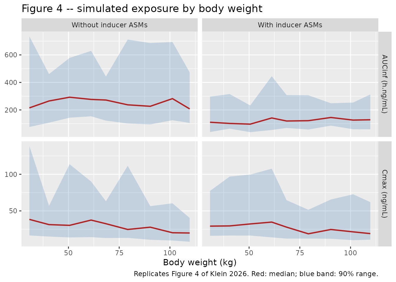
Each claim below is asserted on a per-subject regression across all 200 subjects in a panel, not on the weight-binned medians that the figure plots. A bin median is the median of roughly 22 log-normal draws and carries about 16% standard error, so a bound tight enough to be meaningful on the underlying claim would fail at random on a re-draw; the regression slope over the whole cohort estimates the same quantity an order of magnitude more precisely.
ns  <- per_subject |> filter(panel == "Without inducer ASMs")
ind <- per_subject |> filter(panel == "With inducer ASMs")

# 1. AUCinf carries NO weight effect, because CL is not weight-scaled: the slope
#    of log(AUCinf) on log(WT) must be indistinguishable from zero.
slope_auc <- coef(stats::lm(log(aucinf) ~ log(WT), data = ns))[[2]]
stopifnot(abs(slope_auc) < 0.3)
stopifnot(abs(median(ns$aucinf) / (dose_ug / cl_typ) - 1) < 0.15)

# 2. Cmax must FALL with body weight at roughly the allometric exponent, because
#    Vc scales with weight while CL does not. Expected slope: -e_wt_vc_vp = -0.470.
slope_cmax <- coef(stats::lm(log(cmax) ~ log(WT), data = ns))[[2]]
stopifnot(slope_cmax > -0.9, slope_cmax < -0.1)

# 3. The inducer roughly halves AUCinf (the exact 1/1.955 ratio is asserted
#    deterministically in the structural-identity section above)...
stopifnot(abs((median(ind$aucinf) / median(ns$aucinf)) * 1.955 - 1) < 0.25)

# 4. ...and leaves Cmax essentially unchanged, as the paper states explicitly in
#    Results section 3.2: clearance barely affects the early peak.
stopifnot(abs(median(ind$cmax) / median(ns$cmax) - 1) < 0.20)
The simulation reproduces the three claims the authors draw from
Figure 4: AUCinf is flat across the adolescent weight range (no weight
effect on clearance); Cmax rises modestly at the low end of the weight
range, driven by the weight scaling of Vc and
Vp; and co-administration of an enzyme-inducing antiseizure
medication roughly halves AUCinf while leaving Cmax essentially
unchanged.
Assumptions and deviations
-
Reference weight for the allometric term (70 kg).
The paper reports a shared, freely estimated allometric exponent of
0.470 on
VcandVpbut never states the weight it is normalised to. 70 kg is assumed as the rounded standard. The assumption is corroborated rather than merely asserted: withCLunscaled, the allometric term is the only source of a weight effect on terminal half-life, and at 70 kg the model reproduces the observed Table 1 half-lives in both adolescent weight bands to within 5.6%. A reference of 75.5 kg (the pooled mean weight) fits the observedVss/Fslightly better but the half-lives distinctly worse; neither can be excluded from the published material. -
Reading of the
IIVcolumn of Table S3. Taken asomega * 100on each parameter’s own estimation scale, not as the exact log-normal CV%, on the Figure 4 evidence set out above. The two readings differ by about 8% on omega. -
Estimation scale of
F2and of the inducer effect. Neither is stated; both were recovered from the symmetry of their own published 95% CIs, as tabulated in the source-trace section.F2is carried on the logit scale so that individual dose fractions stay inside (0, 1). -
Two dose records per administration. The paper
describes immediate release into the central compartment alongside
first-order depot absorption but does not print its NONMEM dataset. The
F2label (bioavailability of compartment 2 in NONMEM’s numbering, the central compartment for a two-compartment model with a depot) implies dose records into both compartments, which is how the model is encoded. An event table with a single dose record will silently deliver only one of the two absorption arms. -
Covariates screened but not retained. Height, sex,
age, concomitant antiseizure medications other than the strong inducers,
chronic benzodiazepine use, creatinine clearance and alanine
aminotransferase were all screened in the stepwise covariate analysis
and none was retained; no point estimate is published for any of them.
They are recorded in the model’s
covariatesDataExcludedmetadata rather than encoded. Body weight was also tested onCLandQand rejected, so those two parameters are deliberately not weight-scaled. -
Bioavailability is not identifiable. Every
disposition parameter is apparent (
/F).F2partitions the apparent dose between the two absorption arms; it is not an absolute bioavailability. - Virtual cohort demographics. Body weight is drawn from a normal distribution matched to the UP0100 mean and SD and truncated to the observed range; the paper publishes summary statistics only. Race, sex and age are not simulated because no retained covariate depends on them.
-
Adolescent population sizes. The main text reports
84 patients enrolled in ENGAGE-E-001 while Table S1 reports 80 in the PK
modelling dataset; the model’s
populationmetadata records the modelling dataset (N = 99 overall). - No erratum or corrigendum was found for this article (CrossRef
update-toandupdated-byare both empty; a PubMed erratum search returns no records).