Mosunetuzumab exposure-response for efficacy and cytokine release syndrome (Li 2025)
Source:vignettes/articles/Li_2025_mosunetuzumab.Rmd
Li_2025_mosunetuzumab.RmdModel and source
- Citation: Li C-C, Bender B, Wilkins J, Li F, Turner DC, Wang B, Deng R, Vadhavkar S, Li Z, Kwan A, Huang H, Peng K, Penuel E, Huw L-Y, Chanu P, Li C, Yin S, Wei MC. A Novel Step-Up Dosage Regimen for Enhancing the Benefit-to-Risk Ratio of Mosunetuzumab in Relapsed or Refractory Follicular Lymphoma. Clin Pharmacol Ther. 2025;117(2):465-474. doi:10.1002/cpt.3445.
- Article: https://doi.org/10.1002/cpt.3445 (open access; Data S1 holds Tables S1-S12 and Figures S1-S10).
Li 2025 supports the approved intravenous step-up regimen of
mosunetuzumab, a CD20 x CD3 T-cell-engaging bispecific antibody (1 mg on
Cycle 1 Day 1, 2 mg on Day 8, 60 mg on Day 15 and Cycle 2 Day 1, then 30
mg every 3 weeks), with exposure-response (E-R) models from the phase
I/II GO29781 study. PK was not re-estimated: every exposure metric is an
empirical-Bayes prediction from the Bender 2024 population PK model,
packaged as Bender_2024_mosunetuzumab.
-
Efficacy is driven by the two-cycle AUC0-42
(
AUC_MOSUNETUZUMAB) through Emax logistic regressions for investigator-assessed complete response (CR) and objective response (OR). -
Grade >= 2 cytokine release syndrome (CRS) is
driven by the maximum model-predicted CD20 receptor occupancy
(
ROMAX, percent), either over days 0-42 or within each Cycle 1 dosing window, through linear logistic regressions.
The paper contributes eleven static (no ODE, no time dimension) models:
models <- tibble::tribble(
  ~model, ~endpoint, ~exposure, ~source,
  "Li_2025_mosunetuzumab_cr", "CR (INV)", "AUC0-42", "Table S7",
  "Li_2025_mosunetuzumab_orr", "OR (INV)", "AUC0-42", "Table S7",
  "Li_2025_mosunetuzumab_cr_cov", "CR (INV), + aCD20, SPD", "AUC0-42", "Figure S3 (back-solved)",
  "Li_2025_mosunetuzumab_crs_groupa_astct", "Grade >= 2 CRS, ASTCT, Group A", "ROmax 0-42", "Table S12",
  "Li_2025_mosunetuzumab_crs_groupa_lee", "Grade >= 2 CRS, Lee 2014, Group A", "ROmax 0-42", "Table S12",
  "Li_2025_mosunetuzumab_crs_groupb_astct", "Grade >= 2 CRS, ASTCT, Group B", "ROmax 0-42", "Table S12",
  "Li_2025_mosunetuzumab_crs_groupb_lee", "Grade >= 2 CRS, Lee 2014, Group B", "ROmax 0-42", "Table S12",
  "Li_2025_mosunetuzumab_crs_cov", "Grade >= 2 CRS, Group B, + age, histology", "ROmax 0-42", "Figure S4 + Figure S10",
  "Li_2025_mosunetuzumab_crs_stepup1", "Grade >= 2 CRS, ASTCT, after dose 1", "ROmax in window", "Figure 3a (digitised)",
  "Li_2025_mosunetuzumab_crs_stepup2", "Grade >= 2 CRS, ASTCT, after dose 2", "ROmax in window", "Figure 3a (digitised)",
  "Li_2025_mosunetuzumab_crs_fulldose1", "Grade >= 2 CRS, ASTCT, after dose 3", "ROmax in window", "Figure 3a (digitised)"
)
stopifnot(all(models$model %in% nlmixr2lib::modeldb$name))
knitr::kable(models, caption = "Models contributed by Li 2025.")| model | endpoint | exposure | source |
|---|---|---|---|
| Li_2025_mosunetuzumab_cr | CR (INV) | AUC0-42 | Table S7 |
| Li_2025_mosunetuzumab_orr | OR (INV) | AUC0-42 | Table S7 |
| Li_2025_mosunetuzumab_cr_cov | CR (INV), + aCD20, SPD | AUC0-42 | Figure S3 (back-solved) |
| Li_2025_mosunetuzumab_crs_groupa_astct | Grade >= 2 CRS, ASTCT, Group A | ROmax 0-42 | Table S12 |
| Li_2025_mosunetuzumab_crs_groupa_lee | Grade >= 2 CRS, Lee 2014, Group A | ROmax 0-42 | Table S12 |
| Li_2025_mosunetuzumab_crs_groupb_astct | Grade >= 2 CRS, ASTCT, Group B | ROmax 0-42 | Table S12 |
| Li_2025_mosunetuzumab_crs_groupb_lee | Grade >= 2 CRS, Lee 2014, Group B | ROmax 0-42 | Table S12 |
| Li_2025_mosunetuzumab_crs_cov | Grade >= 2 CRS, Group B, + age, histology | ROmax 0-42 | Figure S4 + Figure S10 |
| Li_2025_mosunetuzumab_crs_stepup1 | Grade >= 2 CRS, ASTCT, after dose 1 | ROmax in window | Figure 3a (digitised) |
| Li_2025_mosunetuzumab_crs_stepup2 | Grade >= 2 CRS, ASTCT, after dose 2 | ROmax in window | Figure 3a (digitised) |
| Li_2025_mosunetuzumab_crs_fulldose1 | Grade >= 2 CRS, ASTCT, after dose 3 | ROmax in window | Figure 3a (digitised) |
Population
- Efficacy (Table S10): 159 adults with relapsed/refractory follicular lymphoma (FL) after >= 2 prior systemic therapies; median age 60 (27-90) years, median weight 80.4 kg, 38.4% female, 76.1% White and 15.1% Asian. Seven patients received fixed dosing (Group A, 0.2-2.8 mg q3w) and 152 a Cycle 1 step-up regimen (Group B; 90 in the pivotal B11 cohort at 1/2/60/30 mg). Median sqrt(SPD) 55.4 mm.
- Safety (Table S11): 439 adults with relapsed/refractory B-cell non-Hodgkin lymphoma (NHL; DLBCL 35.8%, FL 37.1%, transformed FL 13.0%, MCL 8.9%, Richter’s syndrome 3.2%); median age 63 (19-96) years, 35.3% female. 418 were ROmax-evaluable (31 in Group A, 387 in Group B). Median ROmax0-42 0.81% in Group A, 7.5% in cohorts B1-B10 and 36% in B11.
Source trace
| Model | Element | Value | Source |
|---|---|---|---|
| all | Emax logistic
logit(p) = beta0 + Emax*AUC/(E50 + AUC)
|
– | Methods, first E-R equation |
| all CRS | Linear logistic
logit(p) = beta0 + beta*ROmax + ...
|
– | Methods, second E-R equation |
_cr |
logite0, emax, lec50
|
-2.58, 3.36, log(9.18) | Table S7, CR row |
_orr |
logite0, emax, lec50
|
-4.76, 6.23, log(3.12) | Table S7, OR row |
_cr_cov |
logite0 |
-6.23 | back-solved from Figure S3 curves |
_cr_cov |
emax, e_acd20_emax
|
7.394, -0.3363 | back-solved from Figure S3 ‘Max CR’ 76.2% / 52.3% |
_cr_cov |
lec50, e_tumsz_e50,
e_acd20_e50
|
log(2.346), 2.207, 0.0061 | back-solved from Figure S3 E90 annotations |
_crs_groupa_astct |
logite0, e_romax_logit
|
-5.89, 1.32 | Table S12, Group A, ASTCT |
_crs_groupa_lee |
logite0, e_romax_logit
|
-2.14, 0.194 | Table S12, Group A, Lee |
_crs_groupb_astct |
logite0, e_romax_logit
|
-2.64, 0.0196 | Table S12, Group B, ASTCT |
_crs_groupb_lee |
logite0, e_romax_logit
|
-2.44, 0.0180 | Table S12, Group B, Lee |
_crs_cov |
e_romax_logit |
log(1.289)/10 | Figure S4, ‘ROmax (day 42, per 10%)’ |
_crs_cov |
e_age_gt64_logit |
log(0.323) | Figure S4, ‘Baseline age (>64 y)’ |
_crs_cov |
e_tumtp_other_nhl_logit |
log(6.193) | Figure S4, ‘Histology: other’ |
_crs_cov |
logite0 |
-2.77 | digitised from the Figure S10 plateaus |
_crs_stepup1 |
logite0, e_romax_logit
|
-4.03, 0.461 | digitised from Figure 3a, 1st dose |
_crs_stepup2 |
logite0, e_romax_logit
|
-3.59, -1.03 | digitised from Figure 3a, 2nd dose |
_crs_fulldose1 |
logite0, e_romax_logit
|
-3.00, 0.0277 | digitised from Figure 3a, 3rd dose |
Each model also carries a placeholder
addSd_<output> = fixed(0.001) because rxode2 needs an
observation declaration; the source likelihood is Bernoulli.
# The Li 2025 models are purely algebraic: no ODE, no dose, no time
# dimension. A covariate grid is swept along a dummy time axis for one
# subject, and the probability output is read back row by row.
solve_static <- function(model_name, covs) {
  n <- max(vapply(covs, length, integer(1)))
  ev <- data.frame(id = 1L, time = seq_len(n), amt = 0, evid = 0L)
  for (nm in names(covs)) ev[[nm]] <- rep_len(covs[[nm]], n)
  s <- as.data.frame(rxode2::rxSolve(
    # The models carry no etas, so only the placeholder residual is zeroed.
    rxode2::zeroRe(rxode2::rxode(readModelDb(model_name)), which = "sigma"),
    events = ev, returnType = "data.frame"
  ))
  stopifnot(nrow(s) == n)
  s
}
Virtual cohort and exposure metrics
The exposure metrics are re-derived here from
Bender_2024_mosunetuzumab, whose auc state
read at day 42 is AUC0-42 and whose RO output is the
competitive CD20 receptor occupancy (%). Three regimens are simulated,
as in Li 2025 Figure 4: the approved 1/2/60/30 mg, the 1/2/13.5 mg B7
expansion regimen, and a hypothetical 1/2/30 mg regimen without the 60
mg loading doses. Over days 0-42 the doses are Day 1, 8, 15 and Cycle 2
Day 1 (t = 0, 7, 14, 21 days). The covariate distributions follow the
Bender 2024 safety population, as in the
Bender_2024_mosunetuzumab vignette.
# set.seed() seeds R's RNG, used by the covariate draws. It does NOT seed
# rxode2's simulation RNG, whose streams are partitioned per solver thread, so
# the cohort differs between machines with different thread counts. Every
# cohort-based assertion below is on a median, with headroom.
set.seed(20250117)
rxode2::rxSetSeed(20250117)

n_per_arm <- 200L
regimens <- list(
  "1/2/60/30 mg" = c(1, 2, 60, 60),
  "1/2/30 mg" = c(1, 2, 30, 30),
  "1/2/13.5 mg" = c(1, 2, 13.5, 13.5)
)
dose_times <- c(0, 7, 14, 21)

make_covariates <- function(n, id_offset) {
  d <- tibble::tibble(
    id = id_offset + seq_len(n),
    WT = pmin(pmax(stats::rlnorm(n, log(78), 0.22), 37.1), 163),
    ALB = pmin(pmax(stats::rnorm(n, 39, 5.5), 19), 50),
    SEXF = stats::rbinom(n, 1L, 0.353),
    TUMSZ = pmin(pmax(stats::rlnorm(n, log(2970), 0.94), 96), 70900),
    # 44.4% carry detectable rituximab, the rest sit at the 0.5 ug/mL LOQ;
    # 8.0% carry detectable obinutuzumab (Bender 2024 Table 1).
    CP_RITUXIMAB_UGML = ifelse(stats::rbinom(n, 1L, 0.444) == 1L,
                               pmin(stats::rlnorm(n, log(10), 1.1), 151), 0.5),
    CP_OBINUTUZUMAB_UGML = ifelse(stats::rbinom(n, 1L, 0.080) == 1L,
                                  pmin(stats::rlnorm(n, log(10), 1.3), 305), 0)
  )
  d$CP_ACD20_UGML <- pmax(d$CP_RITUXIMAB_UGML, d$CP_OBINUTUZUMAB_UGML)
  d
}

# RO% peaks at the instant of each IV bolus, so the grid includes a point
# just after every dose; ROmax would otherwise be a sampling artefact. An
# observation at exactly a later dose time is recorded after that dose, so
# those times are replaced by points just before and just after the dose;
# otherwise a trapezoidal AUC would ramp linearly up to the post-dose value.
obs_times <- sort(unique(c(
  setdiff(seq(0, 42, by = 0.25), dose_times[-1]),
  dose_times[-1] - 1e-6,
  dose_times + 1e-6
)))

events <- dplyr::bind_rows(lapply(seq_along(regimens), function(i) {
  cov <- make_covariates(n_per_arm, id_offset = (i - 1L) * n_per_arm)
  rxode2::et(amt = regimens[[i]], time = dose_times, cmt = "central") |>
    rxode2::et(obs_times, cmt = "central") |>
    as.data.frame() |>
    dplyr::select(-dplyr::any_of("id")) |>
    tidyr::crossing(cov) |>
    dplyr::mutate(treatment = names(regimens)[i])
})) |>
  dplyr::arrange(id, time, dplyr::desc(evid))
stopifnot(dplyr::n_distinct(events$id) == 3L * n_per_arm)

sim_pk <- rxode2::rxSolve(
  readModelDb("Bender_2024_mosunetuzumab"),
  events,
  keep = c("treatment", "TUMSZ", "CP_ACD20_UGML"),
  returnType = "data.frame"
)
#> ℹ parameter labels from comments will be replaced by 'label()'
exposure <- sim_pk |>
  dplyr::group_by(id, treatment, TUMSZ, CP_ACD20_UGML) |>
  dplyr::summarise(
    AUC_MOSUNETUZUMAB = auc[which.min(abs(time - 42))],
    ROMAX = max(RO[time <= 42]),
    ROMAX_dose1 = max(RO[time < 7]),
    ROMAX_dose2 = max(RO[time >= 7 & time < 14]),
    ROMAX_dose3 = max(RO[time >= 14 & time < 21]),
    .groups = "drop"
  )

exposure_summary <- exposure |>
  dplyr::group_by(treatment) |>
  dplyr::summarise(
    dplyr::across(c(AUC_MOSUNETUZUMAB, ROMAX, ROMAX_dose1, ROMAX_dose2, ROMAX_dose3), median),
    .groups = "drop"
  )
exposure_summary |>
  dplyr::rename(
    Regimen = treatment, `AUC0-42 (day*ug/mL)` = AUC_MOSUNETUZUMAB,
    `ROmax 0-42 (%)` = ROMAX, `ROmax dose 1 (%)` = ROMAX_dose1,
    `ROmax dose 2 (%)` = ROMAX_dose2, `ROmax dose 3 (%)` = ROMAX_dose3
  ) |>
knitr::kable(digits = 2, caption = "Median simulated exposure metrics by regimen.")| Regimen | AUC0-42 (day*ug/mL) | ROmax 0-42 (%) | ROmax dose 1 (%) | ROmax dose 2 (%) | ROmax dose 3 (%) |
|---|---|---|---|---|---|
| 1/2/13.5 mg | 31.32 | 14.37 | 0.76 | 1.83 | 11.54 |
| 1/2/30 mg | 63.65 | 21.47 | 0.59 | 1.35 | 17.33 |
| 1/2/60/30 mg | 129.32 | 41.45 | 0.73 | 1.74 | 34.26 |
b11 <- exposure_summary[exposure_summary$treatment == "1/2/60/30 mg", ]
stopifnot(
  # Li 2025 Table S10: median AUC0-42 145 day*ug/mL in cohort B11 (FL).
  abs(b11$AUC_MOSUNETUZUMAB / 145 - 1) < 0.25,
  # Li 2025 Table S11: median ROmax0-42 36% in cohort B11 (NHL).
  abs(b11$ROMAX / 36 - 1) < 0.30
)
The simulated B11 medians are close to the observed medians of Tables S10 and S11. The per-window maxima reproduce the x-ranges of Figure 3: below about 2.5% after the first two step-up doses and up to about 60% after the third.
Efficacy: CR and OR (Figure 2, Table S7)
auc_grid <- exp(seq(log(0.4), log(251), length.out = 200))
cr_curve <- solve_static("Li_2025_mosunetuzumab_cr", list(AUC_MOSUNETUZUMAB = auc_grid))
orr_curve <- solve_static("Li_2025_mosunetuzumab_orr", list(AUC_MOSUNETUZUMAB = auc_grid))
eff_curves <- dplyr::bind_rows(
  data.frame(auc = auc_grid, p = cr_curve$prob_cr_investigator, endpoint = "(a) Complete response"),
  data.frame(auc = auc_grid, p = orr_curve$prob_orr_investigator, endpoint = "(b) Objective response")
)
auc_ranges <- exposure |>
  dplyr::group_by(treatment) |>
  dplyr::summarise(lo = quantile(AUC_MOSUNETUZUMAB, 0.025), med = median(AUC_MOSUNETUZUMAB),
                   hi = quantile(AUC_MOSUNETUZUMAB, 0.975), .groups = "drop") |>
  dplyr::mutate(y = c(0.02, 0.06, 0.10)[match(treatment, names(regimens))])

ggplot(eff_curves, aes(auc, p)) +
  geom_line(colour = "darkorange", linewidth = 1) +
  geom_errorbar(data = tidyr::crossing(auc_ranges, endpoint = unique(eff_curves$endpoint)),
                aes(y = y, xmin = lo, xmax = hi, colour = treatment), width = 0.02,
                orientation = "y", inherit.aes = FALSE) +
  geom_point(data = tidyr::crossing(auc_ranges, endpoint = unique(eff_curves$endpoint)),
             aes(x = med, y = y, colour = treatment), inherit.aes = FALSE) +
  facet_wrap(~endpoint) +
  scale_x_log10() +
  coord_cartesian(ylim = c(0, 1)) +
  labs(x = "AUC0-42 (day*ug/mL)", y = "Probability of response", colour = "Simulated AUC0-42 (median, 95% range)",
       caption = "Replicates Figure 2 of Li 2025.") +
  theme(legend.position = "bottom")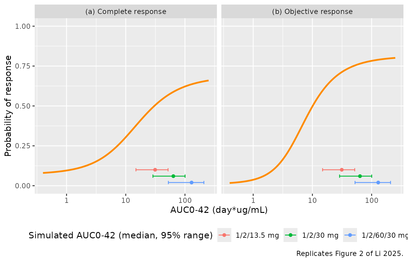
Table S7 derives the maximal response as
expit(beta0 + Emax), and the Results quote the E90 (the
AUC0-42 giving 90% of that maximal probability). Both follow from the
packaged parameters exactly:
e90 <- function(b0, emax, e50) {
  pmax_ <- plogis(b0 + emax)
  frac <- (qlogis(0.9 * pmax_) - b0) / emax
  e50 * frac / (1 - frac)
}
ini_val <- function(model_name, par) {
  df <- rxode2::rxode(readModelDb(model_name))$iniDf
  df$est[df$name == par]
}
eff_check <- tibble::tibble(
  endpoint = c("CR", "OR"),
  model = c("Li_2025_mosunetuzumab_cr", "Li_2025_mosunetuzumab_orr"),
  published_max = c(0.686, 0.814),
  published_e90 = c(92.7, 38.4)
) |>
  dplyr::rowwise() |>
  dplyr::mutate(
    b0 = ini_val(model, "logite0"), emax = ini_val(model, "emax"), e50 = exp(ini_val(model, "lec50")),
    model_max = plogis(b0 + emax),
    model_e90 = e90(b0, emax, e50)
  ) |>
  dplyr::ungroup()
eff_check |>
  dplyr::select(endpoint, published_max, model_max, published_e90, model_e90) |>
  dplyr::rename(Endpoint = endpoint, `Max response (Table S7)` = published_max,
                `Max response (model)` = model_max, `E90 (Results)` = published_e90,
                `E90 (model)` = model_e90) |>
knitr::kable(digits = 3, caption = "Maximal response and E90 versus Li 2025.")| Endpoint | Max response (Table S7) | Max response (model) | E90 (Results) | E90 (model) |
|---|---|---|---|---|
| CR | 0.686 | 0.686 | 92.7 | 92.722 |
| OR | 0.814 | 0.813 | 38.4 | 38.549 |
stopifnot(
  # Deterministic: the bound is the rounding of the published values.
  all(abs(eff_check$model_max - eff_check$published_max) < 0.001),
  all(abs(eff_check$model_e90 / eff_check$published_e90 - 1) < 0.02)
)
Both maximal responses and both E90 values are reproduced to within the rounding of the three printed coefficients (OR E90 38.5 versus 38.4).
Integrated benefit-risk by regimen (Figure 4)
Figure 4 overlays the base CR and OR models with the Group B ASTCT CRS model (the base models, without covariates) over simulated PK profiles at each regimen.
pred <- exposure |>
  dplyr::mutate(
    CR = solve_static("Li_2025_mosunetuzumab_cr", list(AUC_MOSUNETUZUMAB = AUC_MOSUNETUZUMAB))$prob_cr_investigator,
    OR = solve_static("Li_2025_mosunetuzumab_orr", list(AUC_MOSUNETUZUMAB = AUC_MOSUNETUZUMAB))$prob_orr_investigator,
    CRS = solve_static("Li_2025_mosunetuzumab_crs_groupb_astct", list(ROMAX = ROMAX))$prob_crs_grade2
  )

fig4 <- pred |>
  tidyr::pivot_longer(c(CR, OR, CRS), names_to = "endpoint", values_to = "p") |>
  dplyr::group_by(treatment, endpoint) |>
  dplyr::summarise(simulated = 100 * median(p), .groups = "drop") |>
  dplyr::left_join(
    tibble::tribble(
      ~treatment, ~endpoint, ~published,
      "1/2/60/30 mg", "CR", 63.1, "1/2/60/30 mg", "OR", 79.1, "1/2/60/30 mg", "CRS", 11.8,
      "1/2/30 mg", "CR", 58.3, "1/2/30 mg", "OR", 76.4, "1/2/30 mg", "CRS", 9.75,
      "1/2/13.5 mg", "CR", 50.2, "1/2/13.5 mg", "OR", 71.0, "1/2/13.5 mg", "CRS", 8.27
    ),
    by = c("treatment", "endpoint")
  ) |>
  dplyr::mutate(difference = simulated - published)

fig4 |>
  dplyr::rename(Regimen = treatment, Endpoint = endpoint, `Simulated median (%)` = simulated,
                `Li 2025 Figure 4 median (%)` = published, `Difference (points)` = difference) |>
knitr::kable(digits = 1, caption = "Median predicted probability by regimen versus Li 2025 Figure 4.")| Regimen | Endpoint | Simulated median (%) | Li 2025 Figure 4 median (%) | Difference (points) |
|---|---|---|---|---|
| 1/2/13.5 mg | CR | 50.5 | 50.2 | 0.3 |
| 1/2/13.5 mg | CRS | 8.6 | 8.3 | 0.4 |
| 1/2/13.5 mg | OR | 71.2 | 71.0 | 0.2 |
| 1/2/30 mg | CR | 58.8 | 58.3 | 0.5 |
| 1/2/30 mg | CRS | 9.8 | 9.8 | 0.1 |
| 1/2/30 mg | OR | 76.5 | 76.4 | 0.1 |
| 1/2/60/30 mg | CR | 63.6 | 63.1 | 0.5 |
| 1/2/60/30 mg | CRS | 13.9 | 11.8 | 2.1 |
| 1/2/60/30 mg | OR | 79.0 | 79.1 | -0.1 |
ggplot(pred |> tidyr::pivot_longer(c(CR, OR, CRS), names_to = "endpoint", values_to = "p"),
       aes(factor(treatment, levels = rev(names(regimens))), 100 * p, fill = endpoint)) +
  geom_boxplot(outlier.size = 0.5) +
  geom_point(data = fig4, aes(y = published, group = endpoint), shape = 23, size = 2.5,
             fill = "white", position = position_dodge(width = 0.75)) +
  labs(x = "Regimen", y = "Predicted probability (%)", fill = NULL,
       caption = "Replicates Figure 4 of Li 2025 (diamonds: published medians).") +
  theme(legend.position = "bottom")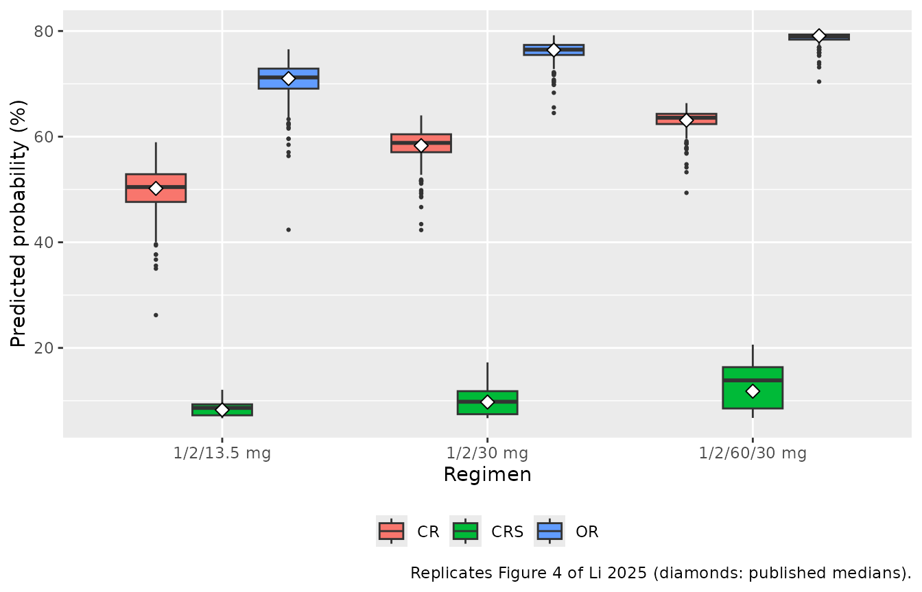
stopifnot(
  # Cohort medians; the efficacy curves are near their plateau at these
  # exposures, so CR/OR medians move little between cohorts. ROmax depends on
  # the residual anti-CD20 mix of the cohort, so CRS gets more headroom.
  all(abs(fig4$difference[fig4$endpoint != "CRS"]) < 4),
  all(abs(fig4$difference[fig4$endpoint == "CRS"]) < 5)
)
The CR and OR medians match Figure 4 to within about one percentage point. The CRS medians are slightly higher than published at the approved regimen, because the simulated ROmax0-42 median of the virtual cohort sits a few points above the observed B11 median of 36%; the ranking of the three regimens and the “< 12%” headline at 1/2/60/30 mg are reproduced to within about two points.
Grade >= 2 CRS over days 0-42 (Figure S9, Table S12)
crs_fits <- tibble::tribble(
  ~model, ~group, ~grading, ~ro_max, ~published_or,
  "Li_2025_mosunetuzumab_crs_groupa_astct", "Group A (fixed dosing)", "ASTCT", 3.43, 3.74,
  "Li_2025_mosunetuzumab_crs_groupa_lee", "Group A (fixed dosing)", "Lee 2014", 3.43, 1.21,
  "Li_2025_mosunetuzumab_crs_groupb_astct", "Group B (step-up dosing)", "ASTCT", 64.3, 1.02,
  "Li_2025_mosunetuzumab_crs_groupb_lee", "Group B (step-up dosing)", "Lee 2014", 64.3, 1.02
)
s9 <- dplyr::bind_rows(lapply(seq_len(nrow(crs_fits)), function(i) {
  ro <- seq(0, crs_fits$ro_max[i], length.out = 100)
  data.frame(ROMAX = ro, group = crs_fits$group[i], grading = crs_fits$grading[i],
             p = solve_static(crs_fits$model[i], list(ROMAX = ro))$prob_crs_grade2)
}))
ggplot(s9, aes(ROMAX, p)) +
  geom_line(colour = "darkorange", linewidth = 1) +
  facet_grid(grading ~ group, scales = "free_x") +
  labs(x = "ROmax0-42 (%)", y = "Probability of grade >= 2 CRS",
       caption = "Replicates the fitted curves of Figure S9 of Li 2025 (x-range: Table S11 ROmax range of each group).")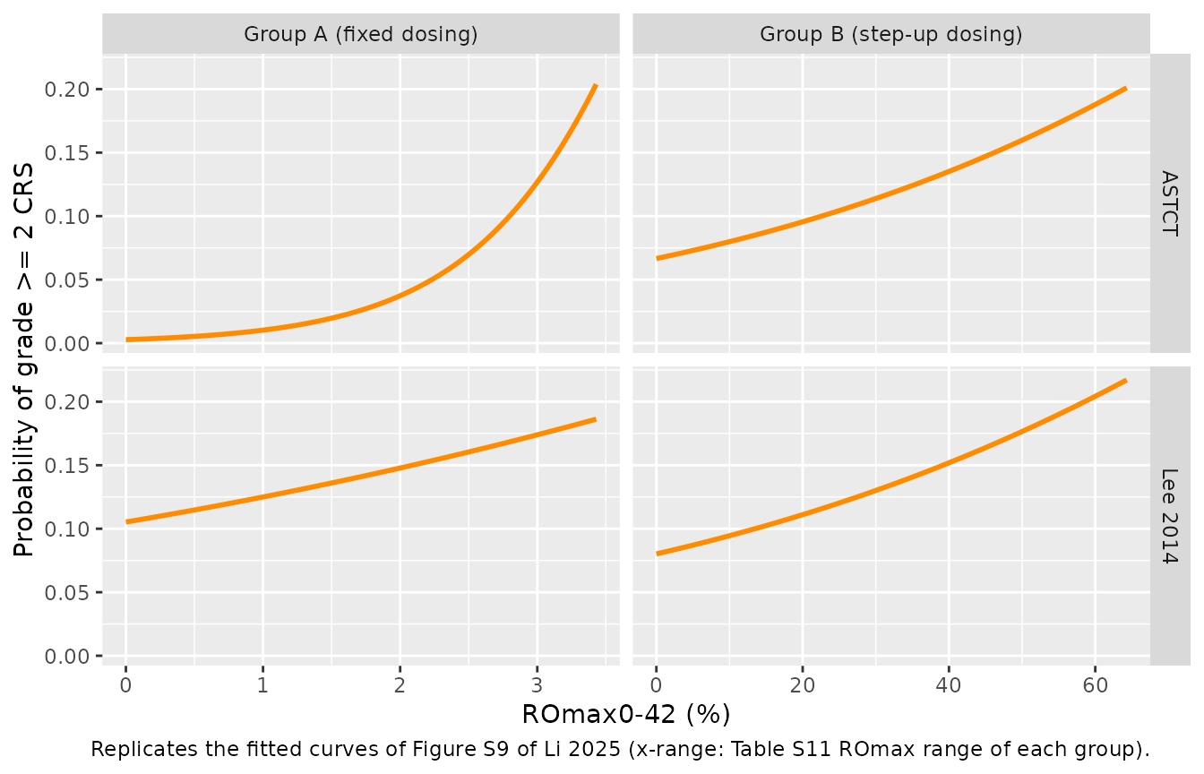
crs_fits$model_or <- vapply(crs_fits$model, function(m) exp(ini_val(m, "e_romax_logit")), numeric(1))
crs_fits |>
  dplyr::select(group, grading, published_or, model_or) |>
  dplyr::rename(Group = group, Grading = grading, `OR per 1% (Table S12)` = published_or,
                `OR per 1% (model)` = model_or) |>
knitr::kable(digits = 3, caption = "Odds ratio per 1% ROmax: Table S12 versus exp(slope).")| Group | Grading | OR per 1% (Table S12) | OR per 1% (model) |
|---|---|---|---|
| Group A (fixed dosing) | ASTCT | 3.74 | 3.743 |
| Group A (fixed dosing) | Lee 2014 | 1.21 | 1.214 |
| Group B (step-up dosing) | ASTCT | 1.02 | 1.020 |
| Group B (step-up dosing) | Lee 2014 | 1.02 | 1.018 |
The positive E-R relationship under fixed dosing (Group A, odds ratio 3.74 per 1% ROmax, not significant) flattens to 1.02 per 1% with step-up dosing, which allowed escalation to more than 20-fold higher occupancy.
Grade >= 2 CRS by dosing window (Figure 3a)
win <- tibble::tribble(
  ~model, ~output, ~window, ~lo, ~hi,
  "Li_2025_mosunetuzumab_crs_stepup1", "prob_crs_stepup1_grade2", "1st dose", 0.031, 2.4,
  "Li_2025_mosunetuzumab_crs_stepup2", "prob_crs_stepup2_grade2", "2nd dose", 0.015, 4.5,
  "Li_2025_mosunetuzumab_crs_fulldose1", "prob_crs_fulldose1_grade2", "3rd dose", 0.051, 59
)
f3a <- dplyr::bind_rows(lapply(seq_len(nrow(win)), function(i) {
  ro <- exp(seq(log(win$lo[i]), log(win$hi[i]), length.out = 100))
  data.frame(ROMAX = ro, window = win$window[i],
             p = solve_static(win$model[i], list(ROMAX = ro))[[win$output[i]]])
}))
b11_windows <- exposure |>
  dplyr::filter(treatment == "1/2/60/30 mg") |>
  dplyr::summarise(`1st dose` = median(ROMAX_dose1), `2nd dose` = median(ROMAX_dose2),
                   `3rd dose` = median(ROMAX_dose3)) |>
  tidyr::pivot_longer(dplyr::everything(), names_to = "window", values_to = "ROMAX")

ggplot(f3a, aes(ROMAX, p, colour = window)) +
  geom_line(linewidth = 1) +
  geom_vline(data = b11_windows, aes(xintercept = ROMAX, colour = window), linetype = 2) +
  scale_x_log10() +
  coord_cartesian(ylim = c(0, 0.4)) +
  labs(x = "ROmax within the dosing window (%)", y = "Probability of grade >= 2 CRS", colour = NULL,
       caption = "Replicates Figure 3a of Li 2025; dashed lines: simulated median ROmax per window at 1/2/60/30 mg.") +
  theme(legend.position = "bottom")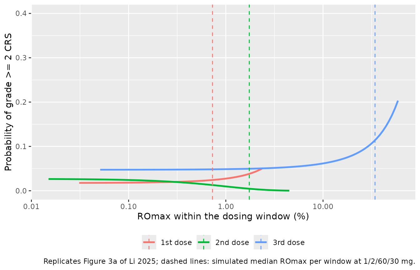
# The coefficients were least-squares fitted to the pixel-traced curve; the
# traced end points are an exact check that the fit reproduces the drawing.
traced <- tibble::tribble(
  ~model, ~output, ~ROMAX, ~traced_p,
  "Li_2025_mosunetuzumab_crs_stepup1", "prob_crs_stepup1_grade2", 0.0312, 0.0172,
  "Li_2025_mosunetuzumab_crs_stepup1", "prob_crs_stepup1_grade2", 2.116, 0.0437,
  "Li_2025_mosunetuzumab_crs_stepup2", "prob_crs_stepup2_grade2", 0.0151, 0.0263,
  "Li_2025_mosunetuzumab_crs_stepup2", "prob_crs_stepup2_grade2", 1.379, 0.0063,
  "Li_2025_mosunetuzumab_crs_fulldose1", "prob_crs_fulldose1_grade2", 0.0511, 0.0476,
  "Li_2025_mosunetuzumab_crs_fulldose1", "prob_crs_fulldose1_grade2", 31.56, 0.1076,
  "Li_2025_mosunetuzumab_crs_fulldose1", "prob_crs_fulldose1_grade2", 59.02, 0.2019
)
traced$model_p <- vapply(seq_len(nrow(traced)), function(i)
  solve_static(traced$model[i], list(ROMAX = traced$ROMAX[i]))[[traced$output[i]]], numeric(1))
knitr::kable(traced[, c("model", "ROMAX", "traced_p", "model_p")], digits = 4,
caption = "Pixel-traced Figure 3a points versus the packaged models.")| model | ROMAX | traced_p | model_p |
|---|---|---|---|
| Li_2025_mosunetuzumab_crs_stepup1 | 0.0312 | 0.0172 | 0.0177 |
| Li_2025_mosunetuzumab_crs_stepup1 | 2.1160 | 0.0437 | 0.0450 |
| Li_2025_mosunetuzumab_crs_stepup2 | 0.0151 | 0.0263 | 0.0265 |
| Li_2025_mosunetuzumab_crs_stepup2 | 1.3790 | 0.0063 | 0.0066 |
| Li_2025_mosunetuzumab_crs_fulldose1 | 0.0511 | 0.0476 | 0.0475 |
| Li_2025_mosunetuzumab_crs_fulldose1 | 31.5600 | 0.1076 | 0.1066 |
| Li_2025_mosunetuzumab_crs_fulldose1 | 59.0200 | 0.2019 | 0.2034 |
# One pixel of Figure 3a is 0.0025 in probability.
stopifnot(all(abs(traced$model_p - traced$traced_p) < 0.003))
The curves shift to the right with each dose: CRS risk at the third (first full) dose stays near 5% until ROmax exceeds about 10%, and the occupancy reached by each dose of the approved regimen sits at the bottom of the corresponding curve.
Covariate model for grade >= 2 CRS (Figures S4 and S10)
s10 <- tidyr::crossing(
  ROMAX = exp(seq(log(0.03), log(64.3), length.out = 100)),
  AGE_GT64 = 0:1, TUMTP_OTHER_NHL = 0:1
)
s10$p <- solve_static("Li_2025_mosunetuzumab_crs_cov",
                      list(ROMAX = s10$ROMAX, AGE_GT64 = s10$AGE_GT64,
                           TUMTP_OTHER_NHL = s10$TUMTP_OTHER_NHL))$prob_crs_grade2
s10 <- s10 |>
  dplyr::mutate(histology = ifelse(TUMTP_OTHER_NHL == 1, "Other", "DLBCL/trFL/FL"),
                age = ifelse(AGE_GT64 == 1, "> 64 y", "<= 64 y"))
ggplot(s10, aes(ROMAX, p, colour = age)) +
  geom_line(linewidth = 1) +
  facet_wrap(~histology) +
  scale_x_log10() +
  coord_cartesian(ylim = c(0, 1)) +
  labs(x = "ROmax0-42 (%)", y = "Probability of grade >= 2 CRS", colour = "Age",
       caption = "Replicates Figure S10 of Li 2025.") +
  theme(legend.position = "bottom")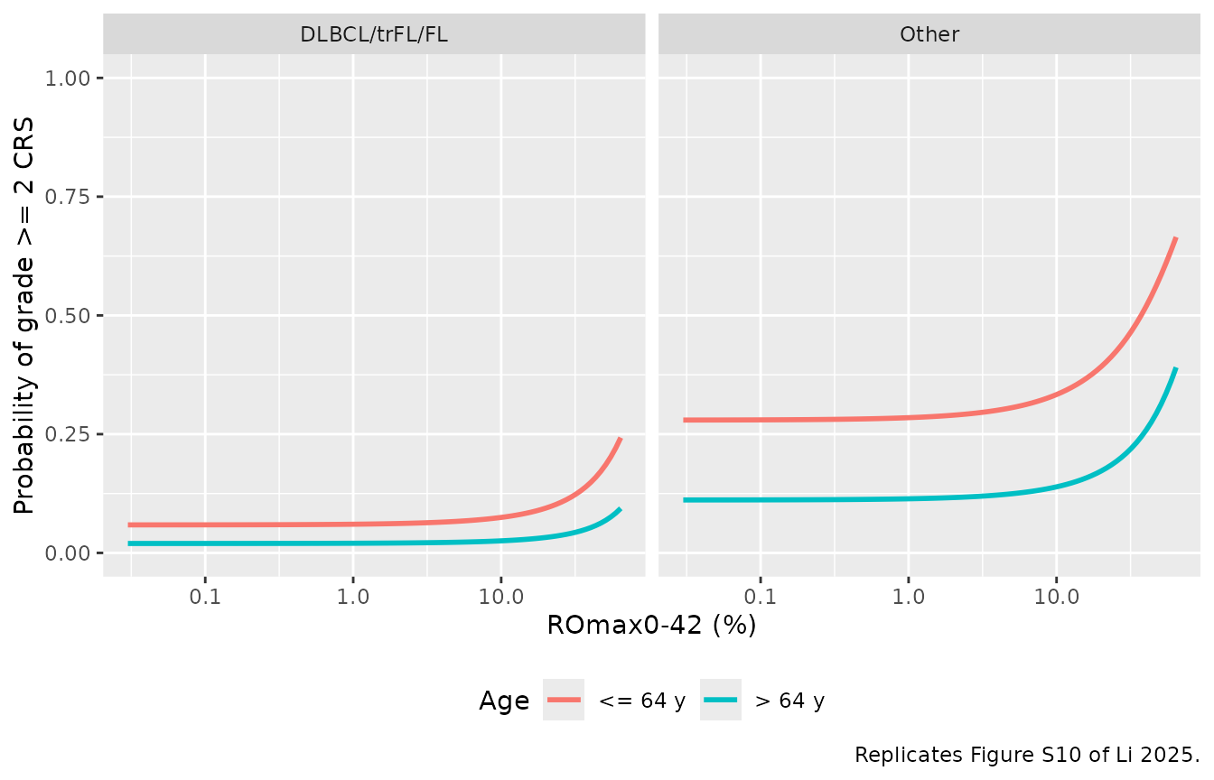
plateau <- s10 |>
  dplyr::filter(ROMAX == min(ROMAX)) |>
  dplyr::select(histology, age, p) |>
  dplyr::left_join(
    tibble::tribble(
      ~histology, ~age, ~digitised,
      "DLBCL/trFL/FL", "<= 64 y", 0.0595, "DLBCL/trFL/FL", "> 64 y", 0.0194,
      "Other", "<= 64 y", 0.2851, "Other", "> 64 y", 0.1096
    ),
    by = c("histology", "age")
  )
knitr::kable(plateau, digits = 4, caption = "Low-ROmax plateau: model versus Figure S10 (pixel-traced).")| histology | age | p | digitised |
|---|---|---|---|
| DLBCL/trFL/FL | <= 64 y | 0.0590 | 0.0595 |
| Other | <= 64 y | 0.2797 | 0.2851 |
| DLBCL/trFL/FL | > 64 y | 0.0199 | 0.0194 |
| Other | > 64 y | 0.1115 | 0.1096 |
# The intercept is the mean of four plateau-derived estimates; the odds ratios
# are the printed Figure S4 values, so each stratum is matched to within the
# spread of those four estimates (0.05 logit) plus the drawing resolution.
stopifnot(all(abs(qlogis(plateau$p) - qlogis(plateau$digitised)) < 0.06))
Exploratory covariate model for CR (Figure S3)
Li 2025 prints no coefficients for this model; the packaged values were back-solved from the Figure S3 annotations and fitted curves (see the model file). The six panels are reproduced here, and the twelve annotations are checked against the packaged model.
s3_grid <- tidyr::crossing(
  CP_ACD20_UGML = c(0.5, 12.1),
  SPDS = c(24.5, 55.4, 104),
  AUC_MOSUNETUZUMAB = exp(seq(log(0.4), log(251), length.out = 80))
) |>
  dplyr::mutate(TUMSZ = SPDS^2)
s3_grid$p <- solve_static("Li_2025_mosunetuzumab_cr_cov",
                          as.list(s3_grid[, c("CP_ACD20_UGML", "TUMSZ", "AUC_MOSUNETUZUMAB")]))$prob_cr_investigator
ggplot(s3_grid, aes(AUC_MOSUNETUZUMAB, p)) +
  geom_line(colour = "orangered", linewidth = 1) +
  facet_grid(paste0("SPDS = ", SPDS, " mm") ~ paste0("aCD20 = ", CP_ACD20_UGML * 1000, " ng/mL")) +
  scale_x_log10() +
  coord_cartesian(ylim = c(0, 0.9)) +
  labs(x = "AUC0-42 (day*ug/mL)", y = "Probability of CR", caption = "Replicates Figure S3 of Li 2025.")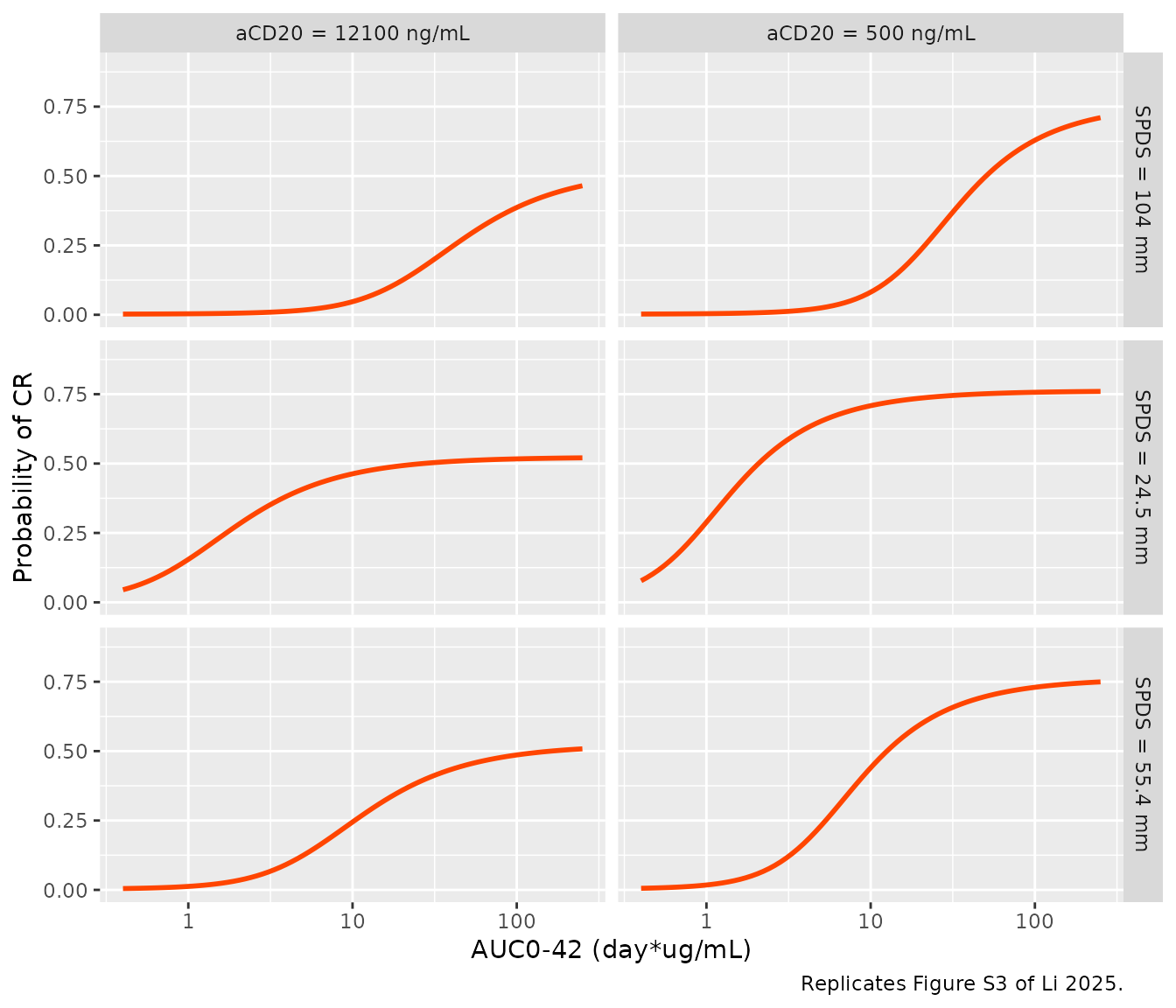
p_cov <- function(par, acd20, spds, auc) {
  emax_i <- par[["emax"]] + par[["e_acd20_emax"]] * log(acd20 / 0.5)
  e50 <- exp(par[["lec50"]]) * (spds / 55.4)^par[["e_tumsz_e50"]] * (acd20 / 0.5)^par[["e_acd20_e50"]]
  plogis(par[["logite0"]] + emax_i * auc / (e50 + auc))
}
ini_cov <- rxode2::rxode(readModelDb("Li_2025_mosunetuzumab_cr_cov"))$iniDf
par_cov <- stats::setNames(ini_cov$est, ini_cov$name)
s3_check <- tibble::tribble(
  ~acd20, ~spds, ~max_cr, ~e90,
  0.5, 24.5, 0.762, 7.07, 0.5, 55.4, 0.762, 42.9, 0.5, 104, 0.762, 173,
  12.1, 24.5, 0.523, 11.7, 12.1, 55.4, 0.523, 68.2, 12.1, 104, 0.523, 283
) |>
  dplyr::rowwise() |>
  dplyr::mutate(
    model_max = p_cov(par_cov, acd20, spds, 1e9),
    model_e90 = stats::uniroot(function(a) p_cov(par_cov, acd20, spds, a) - 0.9 * model_max,
                               c(1e-6, 1e6))$root
  ) |>
  dplyr::ungroup()
# p_cov() restates the model() equations; tie it to the packaged model.
stopifnot(abs(p_cov(par_cov, 12.1, 104, 100) -
                solve_static("Li_2025_mosunetuzumab_cr_cov",
                             list(CP_ACD20_UGML = 12.1, TUMSZ = 104^2, AUC_MOSUNETUZUMAB = 100))$prob_cr_investigator) < 1e-6)
s3_check |>
  dplyr::rename(`aCD20 (ug/mL)` = acd20, `SPDS (mm)` = spds, `Max CR (Fig S3)` = max_cr,
                `Max CR (model)` = model_max, `E90 (Fig S3)` = e90, `E90 (model)` = model_e90) |>
knitr::kable(digits = 3, caption = "Figure S3 annotations versus the back-solved model.")| aCD20 (ug/mL) | SPDS (mm) | Max CR (Fig S3) | E90 (Fig S3) | Max CR (model) | E90 (model) |
|---|---|---|---|---|---|
| 0.5 | 24.5 | 0.762 | 7.07 | 0.762 | 7.090 |
| 0.5 | 55.4 | 0.762 | 42.90 | 0.762 | 42.921 |
| 0.5 | 104.0 | 0.762 | 173.00 | 0.762 | 172.321 |
| 12.1 | 24.5 | 0.523 | 11.70 | 0.523 | 11.533 |
| 12.1 | 55.4 | 0.523 | 68.20 | 0.523 | 69.819 |
| 12.1 | 104.0 | 0.523 | 283.00 | 0.523 | 280.311 |
PKNCA validation of the exposure metric
The efficacy models take AUC0-42 as an input, so the derivation of
that input is checked independently: a PKNCA AUC over days 0-42 of the
simulated concentration profiles must agree with the integrated
auc state, and the cohort exposures are compared with the
published B11 summaries.
sim_nca <- sim_pk |>
  dplyr::filter(!is.na(Cc)) |>
  dplyr::select(id, time, Cc, treatment)
# Guarantee a time-zero record per subject (the pre-dose concentration is 0
# for these first doses; distinct() keeps the simulated post-bolus row if one
# already exists at t = 0).
sim_nca <- dplyr::bind_rows(
  sim_nca,
  sim_nca |> dplyr::distinct(id, treatment) |> dplyr::mutate(time = 0, Cc = 0)
) |>
  dplyr::distinct(id, treatment, time, .keep_all = TRUE) |>
  dplyr::arrange(id, treatment, time)

conc_obj <- PKNCA::PKNCAconc(sim_nca, Cc ~ time | treatment + id)
dose_df <- events |>
  dplyr::filter(evid == 1) |>
  dplyr::select(id, time, amt, treatment)
dose_obj <- PKNCA::PKNCAdose(dose_df, amt ~ time | treatment + id)
intervals <- data.frame(start = 0, end = 42, auclast = TRUE, cmax = TRUE)
nca_res <- PKNCA::pk.nca(PKNCA::PKNCAdata(conc_obj, dose_obj, intervals = intervals))

nca_by_id <- as.data.frame(nca_res) |>
  dplyr::select(id, treatment, PPTESTCD, PPORRES)
auc_check <- nca_by_id |>
  dplyr::filter(PPTESTCD == "auclast") |>
  dplyr::left_join(dplyr::select(exposure, id, AUC_MOSUNETUZUMAB), by = "id") |>
  dplyr::mutate(rel = PPORRES / AUC_MOSUNETUZUMAB - 1)
# Same profiles, two integrators (trapezoid on a 0.25-day grid vs the ODE),
# so the difference is pure numerical error and a tight bound is correct.
stopifnot(abs(median(auc_check$rel)) < 0.01)

published <- tibble::tribble(
  ~treatment, ~auclast, ~cmax,
  "1/2/60/30 mg", 145, 17.9
)
cmp <- nlmixr2lib::ncaComparisonTable(
  simulated = dplyr::select(nca_by_id, treatment, PPTESTCD, PPORRES),
  reference = published,
  by = "treatment",
  units = c(auclast = "day*ug/mL", cmax = "ug/mL"),
  tolerance_pct = 20
)
knitr::kable(cmp, caption = "Simulated cohort medians versus Li 2025 (AUC0-42: Table S10 B11 median; Cmax: Table S5 mean). * marks a difference above 20%.")| NCA parameter | treatment | Reference | Simulated | % diff |
|---|---|---|---|---|
| Cmax (ug/mL) | 1/2/60/30 mg | 17.9 | 14.3 | -20.1%* |
| AUClast (day*ug/mL) | 1/2/60/30 mg | 145 | 129 | -10.8% |
The AUC0-42 reference is the observed B11 median of Table S10. The Cmax reference is the Table S5 arithmetic mean (Cmax over days 0-42, CV 49.6%), which sits above a median for a right-skewed distribution; that is why the simulated median Cmax is flagged at about 20% below it. Table S5 also lists a mean AUC0-42 of 246 dayug/mL for the same regimen, which cannot be reconciled with the 1.59-251 dayug/mL range Table S10 reports for B11 and is not used.
Assumptions and deviations
-
Static models, exposure as input. None of the
eleven models simulates PK;
AUC_MOSUNETUZUMABandROMAXare data columns. Li 2025 derived them from the Bender 2024 popPK model, which is packaged separately (Bender_2024_mosunetuzumab); this vignette derives them the same way. -
Placeholder residual error. Each model carries
addSd_<output> = fixed(0.001)only because rxode2 needs an observation declaration; the source likelihood is Bernoulli. Sample events withrbinom()on the predicted probability. - Figure 3a coefficients are digitised. Li 2025 prints no coefficients for the per-dosing-window CRS models. Each curve of Figure 3a (709 x 261 pixel image) was pixel-traced on the calibrated axes and a logistic linear in untransformed ROmax was least-squares fitted (RMSE below 0.001 in probability). The linear-in-ROmax form follows the Methods equation. The dosing windows are taken as Cycle 1 Day 1 to Day 8, Day 8 to Day 15, and Day 15 to Cycle 2 Day 1; the paper defines them only as “each dosing window”.
- The reduced CRS covariate model intercept is digitised. Figure S4 prints the three odds ratios but not the intercept. It was recovered from the four low-ROmax plateaus of Figure S10 (estimates -2.760, -2.793, -2.743 and -2.789; mean -2.77). The CRS grading scale of this model is not stated; it is presumed to be the ASTCT grading the paper uses for its main CRS results.
-
The exploratory CR covariate model is back-solved, with
assumed forms. Li 2025 prints no coefficients, equations or
reference values for it. Its maximal CR (76.2% / 52.3%) and E90
annotations fix Emax and the six E50 values once beta0 is known. beta0 =
-6.23 was chosen by least squares to the six pixel-traced curves (the
fit is shallow between about -5.5 and -7). The covariate forms are
assumed: the natural-log anti-CD20 concentration of Table S8 enters
linearly in log(aCD20/500 ng/mL) on Emax and on log E50, and sqrt(SPD)
enters as a power on E50 referenced to the 55.4 mm median. The
back-solve found that aCD20 acts almost entirely on Emax (E50 exponent
0.006) and that the SPD exponent is consistent across both aCD20 levels
(2.16-2.26). Only aCD20 = 500 and 12100 ng/mL are constrained by the
source, so predictions between and beyond those levels rest on the
assumed form. Supply
CP_ACD20_UGML = 0.5(the assay LOQ used in the analysis data), not 0, for a patient without quantifiable residual antibody. -
‘Other’ histology.
TUMTP_OTHER_NHLfollows Li 2025’s grouping: MCL, Richter’s syndrome and rarer histologies versus a reference that pools FL, DLBCL and transformed FL. -
Age threshold.
AGE_GT64follows the paper’s ‘<= 64’ / ‘> 64’ years split. - Virtual cohort. The covariate distributions for the Bender 2024 PK simulation (weight, albumin, sex, tumour size, residual rituximab and obinutuzumab) follow the Bender 2024 safety population, not the narrower FL efficacy population, as Li 2025 does not report the distribution it used for the Figure 4 simulations.
- Not extracted. The IFN-gamma versus ROmax relationship of Figure 3b is a LOESS smoother rather than a parametric model, and the progression-free survival and duration-of-response analyses (Figure 5) and the AE-by-tertile analyses (Figure 6, Table S6) are Kaplan-Meier summaries without a fitted model.