N-acetylmannosamine (ManNAc) and Neu5Ac (Van Wart 2021)
Source:vignettes/articles/VanWart_2021_mannac.Rmd
VanWart_2021_mannac.RmdModel and source
#> ℹ parameter labels from comments will be replaced by 'label()'- Citation: Van Wart S, Mager DE, Bednasz CJ, Huizing M, Carrillo N. Population Pharmacokinetic Model of N-acetylmannosamine (ManNAc) and N-acetylneuraminic acid (Neu5Ac) in Subjects with GNE Myopathy. Drugs R D. 2021;21(2):189-202. doi:10.1007/s40268-021-00343-6
- Description: Semi-mechanistic joint population pharmacokinetic model of oral N-acetylmannosamine (ManNAc) and its metabolite N-acetylneuraminic acid (Neu5Ac, sialic acid) in adults with GNE myopathy (Van Wart 2021). ManNAc: one-compartment disposition with first-order absorption after a lag time, relative bioavailability falling with dose as a power function (F = 1 at 6 g), and a constant endogenous ManNAc production that holds the pre-dose baseline M0. Neu5Ac: an indirect-response production through a precursor compartment, both states draining at the Neu5Ac elimination rate constant kout, with production stimulated linearly by plasma ManNAc. The stimulation slope rises exponentially with time from SLP0 to SLPSS (first-order rate kinc), describing the increase in ManNAc-to-Neu5Ac conversion over the first week of dosing. Inter-occasion variability on ManNAc clearance over four occasions. No covariates were retained.
- Article: https://doi.org/10.1007/s40268-021-00343-6
- Supplement (Online Resources 1-10, including the NONMEM control stream of the final model as Online Resource 6): available from the article’s Supplementary Information link.
Van Wart 2021 describes a semi-mechanistic model that fits plasma
N-acetylmannosamine (ManNAc) and its metabolite N-acetylneuraminic acid
(Neu5Ac, sialic acid) jointly, after oral ManNAc in adults with GNE
myopathy, a rare muscle disease caused by deficient sialic acid
biosynthesis. Both species are endogenous, so the model carries baseline
concentrations M0 and N0 that are maintained
before dosing. The authors built the model in four stages as data
accrued (Table 1); the parameters here are those of the Stage 4 final
model (Table 4).
Population
Thirty-four adults with genetically confirmed GNE myopathy contributed data from two NIH studies (Van Wart 2021 Table 2 and Online Resource 1). In the Phase 1 study 12-HG-0207 (NCT01634750), subjects received a single fasting oral dose of 3 g (n = 6), 6 g (n = 8) or 10 g (n = 8) of ManNAc, with placebo in a 3:1 ratio. In the Phase 2 study 15-HG-0068 (NCT02346461), 12 subjects took 3 g or 6 g twice daily for 7 days, then 6 g twice daily for up to 30 months, with a 72-hour washout after Day 90. Eight of them came back at Day 912 and, after a 5-7 day break, took 4 g three times daily. Sixteen subjects were male and 18 female, with a median age of 39.5 years (range 25-65 years) and a median weight of 84.6 kg (range 49.3-115 kg). 70.6% were Caucasian and 26.5% Asian. Renal function was normal (mean cystatin C eGFR 123 mL/min). The analysis used 845 ManNAc and 849 Neu5Ac concentrations.
The same information is available programmatically via
readModelDb("VanWart_2021_mannac")()$population.
Source trace
Every ini() value carries an in-file comment pointing to
its source in
inst/modeldb/specificDrugs/VanWart_2021_mannac.R. The table
below collects them.
| Equation / parameter | Value | Source location |
|---|---|---|
lka (ka) |
0.256 1/h | Table 4 |
lcl (CLM/F) |
631 L/h | Table 4 |
lvc (VM/F) |
506 L | Table 4 |
ltlag (tlag) |
0.254 h | Table 4 |
lrbase (M0) |
61.1 ng/mL | Table 4 |
lrbase_neu5ac (N0) |
150 ng/mL | Table 4 |
lkout_neu5ac (kout) |
0.283 1/h | Table 4 |
lslope0 (SLP0) |
0.000619 mL/ng | Table 4 |
lslope_ss (SLPSS) |
0.00334 mL/ng | Table 4 |
lkinc (kinc) |
0.0287 1/h | Table 4 |
lfdepot |
1 (fixed) | Table 4, ‘F for 6 g dose’ |
e_dose_fdepot |
-0.405 | Table 4, ‘F-Dose slope’; form from Online Resource 6
(F1=(DOSEMG/6000)**THETA(11)) |
etalka, etalcl, etalvc,
etalrbase, etalrbase_neu5ac,
etalslope_ss
|
0.0697, 0.0636, 0.120, 0.0966, 0.0439, 0.383 | Table 4 omega-squared column |
etaiov_cl_1 … etaiov_cl_4
|
0.0580 (shared) | Table 4 ‘IOV on CLM/F’; four occasions from Online Resource 6
$PK
|
propSd (ManNAc) |
sqrt(0.102) = 0.319 | Table 4 ‘sigma2 CCV component’; Online Resource 6
RV_CCV_M
|
propSd_neu5ac (Neu5Ac) |
sqrt(0.0370) = 0.192 | Table 4 row printed ‘Additive component’; Online Resource 6
RV_CCV_N (see Assumptions) |
d/dt(depot) |
n/a | Eq. 1 |
d/dt(central), ksyn = M0 * CLM/F
|
n/a | Eq. 2; Methods 2.3.3 |
d/dt(precursor1),
d/dt(central_neu5ac)
|
n/a | Eqs. 3-4 |
kpro |
n/a | Eq. 5, in the as-run units of Online Resource 6 (see Assumptions) |
slope(t) |
n/a | Eq. 6 |
Initial conditions central(0) = M0 * VM,
precursor1(0) = central_neu5ac(0) = N0
|
n/a | Eqs. 2-4; Online Resource 6 A_INITIAL
|
The model equations are
Structural checks on the typical subject
These checks use the typical-value model (zeroRe()), so
they are deterministic.
mod_typ <- suppressWarnings(rxode2::zeroRe(ui))
th <- ui$theta

# Build one subject's event table. Dose rows carry the dose in DOSE_MANNAC_MG
# (the control stream's DOSEMG); observation rows nominate the ManNAc/Neu5Ac
# endpoint pair with dvid = 1, which returns both Cc and Cc_neu5ac as columns.
# The dose covariate follows id/time/amt/evid/cmt/dvid on purpose.
make_events <- function(id, dose_mg, dose_times, obs_times, occ = 1L) {
  doses <- data.frame(
    id = id, time = dose_times, amt = dose_mg, evid = 1L, cmt = "depot",
    dvid = NA_integer_, DOSE_MANNAC_MG = dose_mg
  )
  obs <- data.frame(
    id = id, time = obs_times, amt = 0, evid = 0L, cmt = NA_character_,
    dvid = 1L, DOSE_MANNAC_MG = 0
  )
  out <- rbind(doses, obs)
  out$OCC <- occ
  out[order(out$id, out$time, -out$evid), ]
}
Secondary parameters of Table 4
Table 4 lists two derived quantities, ksyn and
kpro.
m0 <- exp(th[["lrbase"]])
n0 <- exp(th[["lrbase_neu5ac"]])
cl <- exp(th[["lcl"]])
kout <- exp(th[["lkout_neu5ac"]])
slp0 <- exp(th[["lslope0"]])

ksyn_ugh <- m0 * cl # ng/mL * L/h = ug/h
kpro_eq5 <- kout * n0 / (1 + slp0 * m0) # Eq. 5, M0 in ng/mL
kpro_asrun <- kout * n0 / (1 + slp0 * m0 / 1000) # control stream, M0 in mg/L

derived <- data.frame(
  Quantity = c("ksyn (ug/h)", "kpro, Eq. 5 (ng/mL/h)", "kpro, as run (ng/mL/h)"),
  Model = c(ksyn_ugh, kpro_eq5, kpro_asrun),
  `Table 4` = c(38554, 40.9, 40.9),
  check.names = FALSE
)
knitr::kable(derived, digits = 2, caption = "Derived parameters against Table 4.")| Quantity | Model | Table 4 |
|---|---|---|
| ksyn (ug/h) | 38554.10 | 38554.0 |
| kpro, Eq. 5 (ng/mL/h) | 40.90 | 40.9 |
| kpro, as run (ng/mL/h) | 42.45 | 40.9 |
stopifnot(
  abs(ksyn_ugh / 38554 - 1) < 1e-3,
  # Eq. 5 in consistent units reproduces the printed kpro...
  abs(kpro_eq5 / 40.9 - 1) < 1e-3,
  # ...while the as-run control-stream form is 3.8% higher (see Assumptions).
  abs(kpro_asrun / kpro_eq5 - (1 + slp0 * m0)) < 1e-3
)
ksyn matches exactly. The printed kpro of
40.9 ng/mL/h is Eq. 5 evaluated with M0 in ng/mL. The
fitted control stream evaluates the same expression with M0
in mg/L, which gives 42.45 ng/mL/h. The packaged model keeps that as-run
form, for the reasons given under Assumptions and deviations.
ManNAc: closed-form single-dose solution and relative bioavailability
Plasma ManNAc is linear, with a first-order input after a lag on top
of a constant endogenous baseline. For a single dose the model must
therefore equal the closed form
M(t) = M0 + F * Dose * ka / (V * (ka - k)) * (exp(-k (t - tlag)) - exp(-ka (t - tlag)))
for t > tlag, with F = (Dose / 6 g)^-0.405.
The Results give the fitted F as ranging “from 1.32 at a dose of 3 g to
0.81 at a dose of 10 g”.
ka <- exp(th[["lka"]])
vc <- exp(th[["lvc"]])
tlag <- exp(th[["ltlag"]])
k <- cl / vc
tt <- c(0, 0.1, seq(0.5, 24, by = 0.5))

cf_rows <- lapply(c(3000, 6000, 10000), function(d) {
  s <- rxode2::rxSolve(
    mod_typ, make_events(1L, d, 0, tt),
    returnType = "data.frame", useLinCmt = FALSE, rtol = 1e-10, atol = 1e-12
  )
  f_dose <- (d / 6000)^th[["e_dose_fdepot"]]
  te <- pmax(s$time - tlag, 0)
  cf <- m0 + 1000 * f_dose * d * ka / (vc * (ka - k)) * (exp(-k * te) - exp(-ka * te))
  data.frame(dose_g = d / 1000, F = f_dose, max_rel_err = max(abs(s$Cc / cf - 1)))
})
#> ℹ omega/sigma items treated as zero: 'etalka', 'etalcl', 'etalvc', 'etalrbase', 'etalrbase_neu5ac', 'etalslope_ss', 'etaiov_cl_1', 'etaiov_cl_2', 'etaiov_cl_3', 'etaiov_cl_4'
#> ℹ omega/sigma items treated as zero: 'etalka', 'etalcl', 'etalvc', 'etalrbase', 'etalrbase_neu5ac', 'etalslope_ss', 'etaiov_cl_1', 'etaiov_cl_2', 'etaiov_cl_3', 'etaiov_cl_4'
#> ℹ omega/sigma items treated as zero: 'etalka', 'etalcl', 'etalvc', 'etalrbase', 'etalrbase_neu5ac', 'etalslope_ss', 'etaiov_cl_1', 'etaiov_cl_2', 'etaiov_cl_3', 'etaiov_cl_4'
cf_tab <- do.call(rbind, cf_rows)
knitr::kable(cf_tab, digits = c(0, 3, 12),
caption = "Relative bioavailability and agreement of the ODE solution with the closed form.")| dose_g | F | max_rel_err |
|---|---|---|
| 3 | 1.324 | 7.8e-11 |
| 6 | 1.000 | 9.3e-11 |
| 10 | 0.813 | 8.2e-11 |
Endogenous baselines and the time-dependent conversion slope
With no dose, ManNAc must hold at M0 forever. Neu5Ac
starts at N0, but it does not hold there. The conversion
slope SLP(t) rises from SLP0 towards
SLPSS as a function of time alone (Eq. 6), so an undosed
subject’s Neu5Ac settles at the level set by SLPSS:
N_ss = kpro * (1 + SLPSS * M0) / kout. Online Resource 10
notes that “after about 1 week, the SLP parameter reaches steady-state
levels”.
b <- rxode2::rxSolve(
  mod_typ, make_events(1L, 0, 0, c(0, 24, 168, 336, 2000)),
  returnType = "data.frame", useLinCmt = FALSE, rtol = 1e-10, atol = 1e-12
)
#> ℹ omega/sigma items treated as zero: 'etalka', 'etalcl', 'etalvc', 'etalrbase', 'etalrbase_neu5ac', 'etalslope_ss', 'etaiov_cl_1', 'etaiov_cl_2', 'etaiov_cl_3', 'etaiov_cl_4'
slp_ss <- exp(th[["lslope_ss"]])
n_ss <- kpro_asrun * (1 + slp_ss * m0) / kout
frac_1wk <- (b$slope[b$time == 168] - slp0) / (slp_ss - slp0)

knitr::kable(b[, c("time", "Cc", "Cc_neu5ac", "slope")], digits = 6,
caption = "Undosed typical subject.")| time | Cc | Cc_neu5ac | slope |
|---|---|---|---|
| 0 | 61.1 | 150.0000 | 0.000619 |
| 24 | 61.1 | 165.0739 | 0.001974 |
| 168 | 61.1 | 180.3555 | 0.003318 |
| 336 | 61.1 | 180.6023 | 0.003340 |
| 2000 | 61.1 | 180.6043 | 0.003340 |
stopifnot(
  max(abs(b$Cc / m0 - 1)) < 1e-8,
  abs(b$Cc_neu5ac[b$time == 0] / n0 - 1) < 1e-8,
  abs(b$Cc_neu5ac[b$time == 2000] / n_ss - 1) < 1e-6,
  frac_1wk > 0.99
)
SLP has covered 99.2% of its rise by one week, which
matches Online Resource 10. The undosed Neu5Ac level rises from 150 to
180.6 ng/mL. That rise is built into the published model, not a defect
of the encoding: SLP is a function of time since the start
of the subject’s record, and dosing does not enter it.
Single-dose simulations (Figures 3 and 4)
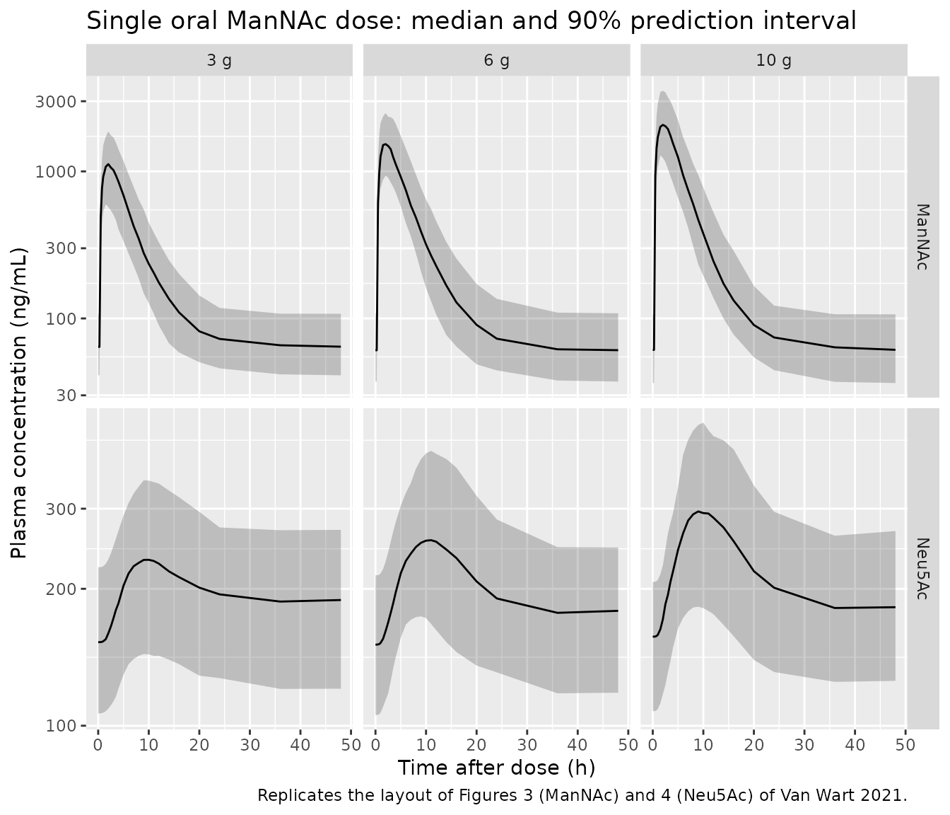
Van Wart 2021 Figures 3 and 4 are VPCs of plasma ManNAc and Neu5Ac after a single 3, 6 or 10 g dose in study 12-HG-0207. The chunk below simulates 100 virtual subjects per dose group with between-subject variability and plots the 5th, 50th and 95th percentiles of the individual predictions. No covariates are needed because none were retained.
rxode2::rxSetSeed(2021)
n_sd <- 100
sd_times <- c(0, 0.25, 0.5, 0.75, 1, 1.5, 2, 2.5, 3, 3.5, 4, 5, 6, 7, 8, 9, 10,
  11, 12, 14, 16, 20, 24, 36, 48)
sd_doses <- c(3000, 6000, 10000)
sd_events <- do.call(rbind, lapply(seq_along(sd_doses), function(i) {
  ev <- do.call(rbind, lapply((i - 1) * n_sd + seq_len(n_sd), function(j) {
    make_events(j, sd_doses[i], 0, sd_times)
  }))
  ev$treatment <- paste0(sd_doses[i] / 1000, " g")
  ev
}))
stopifnot(!anyDuplicated(unique(sd_events[, c("id", "time", "evid")])))

sd_sim <- rxode2::rxSolve(mod, events = sd_events, keep = "treatment",
  returnType = "data.frame", useLinCmt = FALSE)
#> ℹ parameter labels from comments will be replaced by 'label()'
#> Warning: some etas defaulted to non-mu referenced, possible parsing error: etaiov_cl_1, etaiov_cl_2, etaiov_cl_3, etaiov_cl_4
#> as a work-around try putting the mu-referenced expression on a simple line
sd_sim$treatment <- factor(sd_sim$treatment, levels = c("3 g", "6 g", "10 g"))
stopifnot(!anyNA(sd_sim$Cc), !anyNA(sd_sim$Cc_neu5ac))
sd_sim |>
  select(id, time, treatment, ManNAc = Cc, Neu5Ac = Cc_neu5ac) |>
  pivot_longer(c(ManNAc, Neu5Ac), names_to = "analyte", values_to = "conc") |>
  group_by(analyte, treatment, time) |>
  summarise(
    Q05 = quantile(conc, 0.05), Q50 = median(conc), Q95 = quantile(conc, 0.95),
    .groups = "drop"
  ) |>
  ggplot(aes(time, Q50)) +
  geom_ribbon(aes(ymin = Q05, ymax = Q95), alpha = 0.25) +
  geom_line() +
  facet_grid(analyte ~ treatment, scales = "free_y") +
  scale_y_log10() +
  labs(
    x = "Time after dose (h)", y = "Plasma concentration (ng/mL)",
    title = "Single oral ManNAc dose: median and 90% prediction interval",
    caption = "Replicates the layout of Figures 3 (ManNAc) and 4 (Neu5Ac) of Van Wart 2021."
  )
PKNCA: single dose
The Introduction summarises the single-dose Phase 1 data (reference 11 of the paper): ManNAc is “absorbed rapidly (Tmax 2-2.5 h)” and Neu5Ac peaks later (“Tmax 8-11 h”). These are observed values from the same study the model was fitted to. Concentrations include the endogenous baseline, as measured.
sd_dose <- sd_events |>
  filter(evid == 1) |>
  select(id, time, amt, treatment)
sd_int <- data.frame(start = 0, end = 48, cmax = TRUE, tmax = TRUE, auclast = TRUE)

nca_sd <- function(conc_col) {
  conc <- sd_sim |>
    filter(!is.na(.data[[conc_col]])) |>
    transmute(id, time, treatment = as.character(treatment), conc = .data[[conc_col]])
  conc_obj <- PKNCA::PKNCAconc(conc, conc ~ time | treatment + id)
  dose_obj <- PKNCA::PKNCAdose(sd_dose, amt ~ time | treatment + id)
  PKNCA::pk.nca(PKNCA::PKNCAdata(conc_obj, dose_obj, intervals = sd_int))
}
nca_sd_m <- nca_sd("Cc")
nca_sd_n <- nca_sd("Cc_neu5ac")

sd_summary <- bind_rows(
  as.data.frame(nca_sd_m) |> mutate(analyte = "ManNAc"),
  as.data.frame(nca_sd_n) |> mutate(analyte = "Neu5Ac")
) |>
  group_by(analyte, treatment, PPTESTCD) |>
  summarise(median = median(PPORRES), .groups = "drop") |>
  pivot_wider(names_from = PPTESTCD, values_from = median) |>
  mutate(treatment = factor(treatment, levels = c("3 g", "6 g", "10 g"))) |>
  arrange(analyte, treatment)

sd_summary |>
  select(analyte, treatment, cmax, tmax, auclast) |>
  rename(
    "Analyte" = analyte, "Dose" = treatment, "Cmax (ng/mL)" = cmax,
    "Tmax (h)" = tmax, "AUC0-48 (ng*h/mL)" = auclast
  ) |>
knitr::kable(digits = 1, caption = "Median simulated single-dose NCA (100 subjects per dose).")| Analyte | Dose | Cmax (ng/mL) | Tmax (h) | AUC0-48 (ng*h/mL) |
|---|---|---|---|---|
| ManNAc | 3 g | 1159.2 | 2 | 9673.9 |
| ManNAc | 6 g | 1587.8 | 2 | 12198.5 |
| ManNAc | 10 g | 2115.7 | 2 | 15466.3 |
| Neu5Ac | 3 g | 232.9 | 10 | 9520.0 |
| Neu5Ac | 6 g | 255.9 | 10 | 9652.8 |
| Neu5Ac | 10 g | 297.3 | 9 | 10337.3 |
tmax_m <- sd_summary$tmax[sd_summary$analyte == "ManNAc"]
tmax_n <- sd_summary$tmax[sd_summary$analyte == "Neu5Ac"]
stopifnot(
  length(tmax_m) == 3, length(tmax_n) == 3,
  # Introduction: ManNAc Tmax 2-2.5 h and Neu5Ac Tmax 8-11 h across the three
  # dose groups (observed). A 0.5 h grid margin either side allows for the
  # sampling grid and for cohort-to-cohort variation of a median.
  all(tmax_m >= 1.5 & tmax_m <= 3),
  all(tmax_n >= 7.5 & tmax_n <= 11.5)
)
The simulated median Tmax sits inside the reported ranges for both analytes and all three dose groups. The Neu5Ac peak comes about 6-8 hours after the ManNAc peak, as the paper notes.
Repeated dosing (Figures 5 and 6)
Study 15-HG-0068 started with 3 g or 6 g twice daily for 7 days, sampled intensively on Days 1 and 7. Figures 5 and 6 are the repeated-dose VPCs. The occasion switches from 1 to 2 at Day 4, as in the control stream. Neu5Ac rises from Day 1 to Day 7 because the conversion slope increases over the week.
rxode2::rxSetSeed(2022)
n_md <- 100
md_obs <- c(seq(0, 12, by = 0.5), 144 + seq(0, 12, by = 0.5))
md_doses <- c(3000, 6000)
md_events <- do.call(rbind, lapply(seq_along(md_doses), function(i) {
  ev <- do.call(rbind, lapply((i - 1) * n_md + seq_len(n_md), function(j) {
    make_events(j, md_doses[i], seq(0, 156, by = 12), md_obs)
  }))
  ev$OCC <- ifelse(ev$time < 72, 1L, 2L)
  ev$treatment <- paste0(md_doses[i] / 1000, " g BID")
  ev
}))
stopifnot(!anyDuplicated(unique(md_events[, c("id", "time", "evid")])))

md_sim <- rxode2::rxSolve(mod, events = md_events, keep = "treatment",
  returnType = "data.frame", useLinCmt = FALSE)
stopifnot(!anyNA(md_sim$Cc), !anyNA(md_sim$Cc_neu5ac))
md_sim$day <- ifelse(md_sim$time < 72, "Day 1", "Day 7")
md_sim$tad <- ifelse(md_sim$time < 72, md_sim$time, md_sim$time - 144)
md_sim |>
  select(id, tad, day, treatment, ManNAc = Cc, Neu5Ac = Cc_neu5ac) |>
  pivot_longer(c(ManNAc, Neu5Ac), names_to = "analyte", values_to = "conc") |>
  group_by(analyte, treatment, day, tad) |>
  summarise(
    Q05 = quantile(conc, 0.05), Q50 = median(conc), Q95 = quantile(conc, 0.95),
    .groups = "drop"
  ) |>
  ggplot(aes(tad, Q50, colour = day, fill = day)) +
  geom_ribbon(aes(ymin = Q05, ymax = Q95), alpha = 0.15, colour = NA) +
  geom_line() +
  facet_grid(analyte ~ treatment, scales = "free_y") +
  scale_y_log10() +
  labs(
    x = "Time after the morning dose (h)", y = "Plasma concentration (ng/mL)",
    colour = NULL, fill = NULL,
    title = "Twice-daily ManNAc, Days 1 and 7: median and 90% prediction interval",
    caption = "Replicates the layout of Figures 5 (ManNAc) and 6 (Neu5Ac) of Van Wart 2021."
  )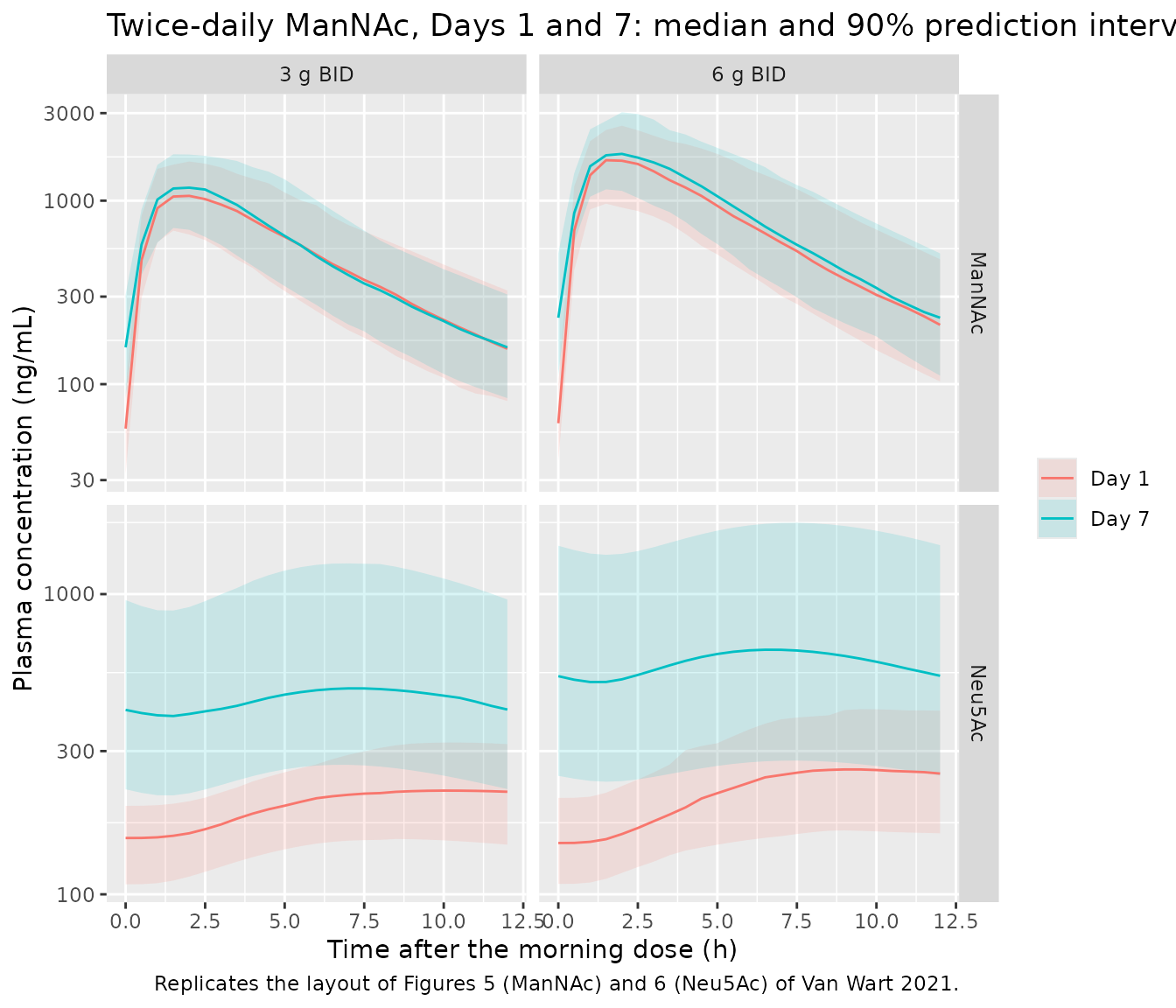
The typical subject makes the Day-1-to-Day-7 increase deterministic:
md_typ <- rxode2::rxSolve(
  mod_typ, make_events(1L, 6000, seq(0, 156, by = 12), md_obs, occ = 1L),
  returnType = "data.frame", useLinCmt = FALSE
)
#> ℹ omega/sigma items treated as zero: 'etalka', 'etalcl', 'etalvc', 'etalrbase', 'etalrbase_neu5ac', 'etalslope_ss', 'etaiov_cl_1', 'etaiov_cl_2', 'etaiov_cl_3', 'etaiov_cl_4'
n_cmax_d1 <- max(md_typ$Cc_neu5ac[md_typ$time <= 12])
n_cmax_d7 <- max(md_typ$Cc_neu5ac[md_typ$time >= 144])
m_cmax_d1 <- max(md_typ$Cc[md_typ$time <= 12])
m_cmax_d7 <- max(md_typ$Cc[md_typ$time >= 144])
c(neu5ac_day7_over_day1 = n_cmax_d7 / n_cmax_d1, mannac_day7_over_day1 = m_cmax_d7 / m_cmax_d1)
#> neu5ac_day7_over_day1 mannac_day7_over_day1
#>              2.554389              1.056885
stopifnot(
  # ManNAc disposition is fast (0.56 h half-life), but absorption is slow
  # (ka = 0.256 1/h, a 2.7 h half-life), so about exp(-0.256 * 11.75) = 5% of
  # each dose is still in the depot at the next dose: slight accumulation only.
  m_cmax_d7 / m_cmax_d1 > 1, m_cmax_d7 / m_cmax_d1 < 1.1,
  # Neu5Ac rises markedly over the week as SLP approaches SLPSS.
  n_cmax_d7 / n_cmax_d1 > 1.5
)
Dosing-regimen simulations (Table 3) and PKNCA
Table 3 gives the median and 5th-95th percentiles of the average
steady-state concentration (Css,ave = AUC over the dosing
interval on Day 30, divided by tau; Online Resource 4) for 3, 4, 6 and
10 g every 8, 12 or 24 hours, with 90 virtual subjects. The paper
simulated “a single clinical trial”, so the same 90 subjects appear in
every regimen. That design is reproduced here with common random
numbers. The 90 subjects’ random effects are drawn once in base R and
passed to the typical-value model as data columns. Every regimen
therefore sees the same subjects, and the result depends only on R’s own
seed, not on rxode2’s thread count. Day 30 falls in occasion 3 of the
IOV structure (Day >= 30), which is used throughout.
set.seed(2021)
n_t3 <- 90
om <- ui$omega
etas <- as.data.frame(matrix(rnorm(n_t3 * ncol(om)), n_t3) %*% chol(om))
names(etas) <- colnames(om)
etas$pid <- seq_len(n_t3)

regimens <- expand.grid(dose_g = c(3, 4, 6, 10), tau = c(8, 12, 24))
regimens$regimen <- sprintf("%g g Q%dH", regimens$dose_g, regimens$tau)
day30 <- 29 * 24

t3_events <- do.call(rbind, lapply(seq_len(nrow(regimens)), function(i) {
  r <- regimens[i, ]
  ev <- do.call(rbind, lapply(seq_len(n_t3), function(p) {
    e <- make_events(
      (i - 1) * n_t3 + p, r$dose_g * 1000,
      seq(0, by = r$tau, length.out = 30 * 24 / r$tau),
      day30 + seq(0, r$tau, by = 0.25), occ = 3L
    )
    e$pid <- p
    e
  }))
  ev$regimen <- r$regimen
  ev
})) |>
  left_join(etas, by = "pid")
stopifnot(!anyDuplicated(unique(t3_events[, c("id", "time", "evid")])))

t3_sim <- rxode2::rxSolve(mod_typ, events = t3_events, keep = "regimen",
  returnType = "data.frame", useLinCmt = FALSE)
#> ℹ omega/sigma items treated as zero: 'etalka', 'etalcl', 'etalvc', 'etalrbase', 'etalrbase_neu5ac', 'etalslope_ss', 'etaiov_cl_1', 'etaiov_cl_2', 'etaiov_cl_3', 'etaiov_cl_4'
#> Warning: multi-subject simulation without without 'omega'
stopifnot(!anyNA(t3_sim$Cc), !anyNA(t3_sim$Cc_neu5ac))
# The etas were applied: the panel's clearances spread around the typical 631 L/h.
stopifnot(sd(log(t3_sim$cl)) > 0.2)
Css,ave is PKNCA’s cav over the Day-30
dosing interval.
t3_dose <- t3_events |>
  filter(evid == 1) |>
  select(id, time, amt, regimen)
t3_int <- regimens |>
  transmute(regimen, start = day30, end = day30 + tau, cav = TRUE)

nca_t3 <- function(conc_col) {
  conc <- t3_sim |>
    filter(!is.na(.data[[conc_col]])) |>
    transmute(id, time, regimen, conc = .data[[conc_col]])
  conc_obj <- PKNCA::PKNCAconc(conc, conc ~ time | regimen + id)
  dose_obj <- PKNCA::PKNCAdose(t3_dose, amt ~ time | regimen + id)
  PKNCA::pk.nca(PKNCA::PKNCAdata(conc_obj, dose_obj, intervals = t3_int))
}
nca_t3_m <- nca_t3("Cc")
nca_t3_n <- nca_t3("Cc_neu5ac")

# Van Wart 2021 Table 3: median and 5th-95th percentiles of Css,ave (ng/mL).
table3 <- tibble::tribble(
  ~analyte, ~regimen, ~t3_median, ~t3_p05, ~t3_p95,
  "ManNAc", "3 g Q8H", 922, 501, 1550,
  "ManNAc", "4 g Q8H", 1060, 573, 1790,
  "ManNAc", "6 g Q8H", 1290, 692, 2180,
  "ManNAc", "10 g Q8H", 1650, 883, 2810,
  "ManNAc", "3 g Q12H", 642, 359, 1060,
  "ManNAc", "4 g Q12H", 729, 404, 1220,
  "ManNAc", "6 g Q12H", 881, 480, 1480,
  "ManNAc", "10 g Q12H", 1120, 607, 1900,
  "ManNAc", "3 g Q24H", 365, 223, 570,
  "ManNAc", "4 g Q24H", 411, 246, 650,
  "ManNAc", "6 g Q24H", 483, 281, 780,
  "ManNAc", "10 g Q24H", 603, 340, 989,
  "Neu5Ac", "3 g Q8H", 633, 247, 2010,
  "Neu5Ac", "4 g Q8H", 702, 265, 2300,
  "Neu5Ac", "6 g Q8H", 818, 296, 2780,
  "Neu5Ac", "10 g Q8H", 1020, 344, 3540,
  "Neu5Ac", "3 g Q12H", 484, 209, 1420,
  "Neu5Ac", "4 g Q12H", 533, 222, 1610,
  "Neu5Ac", "6 g Q12H", 612, 242, 1930,
  "Neu5Ac", "10 g Q12H", 735, 274, 2440,
  "Neu5Ac", "3 g Q24H", 338, 174, 825,
  "Neu5Ac", "4 g Q24H", 364, 181, 921,
  "Neu5Ac", "6 g Q24H", 405, 190, 1080,
  "Neu5Ac", "10 g Q24H", 464, 204, 1330
)

cmp_m <- nlmixr2lib::ncaComparisonTable(
  simulated = nca_t3_m,
  reference = table3 |> filter(analyte == "ManNAc") |> transmute(regimen, cav = t3_median),
  by = "regimen", units = c(cav = "ng/mL"), tolerance_pct = 20
)
cmp_n <- nlmixr2lib::ncaComparisonTable(
  simulated = nca_t3_n,
  reference = table3 |> filter(analyte == "Neu5Ac") |> transmute(regimen, cav = t3_median),
  by = "regimen", units = c(cav = "ng/mL"), tolerance_pct = 20
)
knitr::kable(cmp_m, caption = "Plasma ManNAc Css,ave: simulated median vs. Table 3. * differs by >20%.")| NCA parameter | regimen | Reference | Simulated | % diff |
|---|---|---|---|---|
| Cavg (ng/mL) | 3 g Q8H | 922 | 826 | -10.4% |
| Cavg (ng/mL) | 4 g Q8H | 1060 | 966 | -8.9% |
| Cavg (ng/mL) | 6 g Q8H | 1290 | 1210 | -6.3% |
| Cavg (ng/mL) | 10 g Q8H | 1650 | 1610 | -2.3% |
| Cavg (ng/mL) | 3 g Q12H | 642 | 578 | -10.0% |
| Cavg (ng/mL) | 4 g Q12H | 729 | 670 | -8.1% |
| Cavg (ng/mL) | 6 g Q12H | 881 | 831 | -5.7% |
| Cavg (ng/mL) | 10 g Q12H | 1120 | 1100 | -1.8% |
| Cavg (ng/mL) | 3 g Q24H | 365 | 323 | -11.6% |
| Cavg (ng/mL) | 4 g Q24H | 411 | 373 | -9.1% |
| Cavg (ng/mL) | 6 g Q24H | 483 | 457 | -5.4% |
| Cavg (ng/mL) | 10 g Q24H | 603 | 590 | -2.2% |
knitr::kable(cmp_n, caption = "Plasma Neu5Ac Css,ave: simulated median vs. Table 3. * differs by >20%.")| NCA parameter | regimen | Reference | Simulated | % diff |
|---|---|---|---|---|
| Cavg (ng/mL) | 3 g Q8H | 633 | 561 | -11.4% |
| Cavg (ng/mL) | 4 g Q8H | 702 | 627 | -10.6% |
| Cavg (ng/mL) | 6 g Q8H | 818 | 743 | -9.1% |
| Cavg (ng/mL) | 10 g Q8H | 1020 | 946 | -7.3% |
| Cavg (ng/mL) | 3 g Q12H | 484 | 447 | -7.7% |
| Cavg (ng/mL) | 4 g Q12H | 533 | 490 | -8.0% |
| Cavg (ng/mL) | 6 g Q12H | 612 | 563 | -8.0% |
| Cavg (ng/mL) | 10 g Q12H | 735 | 691 | -6.0% |
| Cavg (ng/mL) | 3 g Q24H | 338 | 309 | -8.6% |
| Cavg (ng/mL) | 4 g Q24H | 364 | 334 | -8.3% |
| Cavg (ng/mL) | 6 g Q24H | 405 | 380 | -6.2% |
| Cavg (ng/mL) | 10 g Q24H | 464 | 453 | -2.4% |
The comparison tables give the medians. The 90% intervals come from the same PKNCA results:
t3_pct <- bind_rows(
  as.data.frame(nca_t3_m) |> mutate(analyte = "ManNAc"),
  as.data.frame(nca_t3_n) |> mutate(analyte = "Neu5Ac")
) |>
  filter(PPTESTCD == "cav") |>
  group_by(analyte, regimen) |>
  summarise(
    median = median(PPORRES), p05 = quantile(PPORRES, 0.05), p95 = quantile(PPORRES, 0.95),
    .groups = "drop"
  ) |>
  left_join(table3, by = c("analyte", "regimen")) |>
  mutate(
    pct_diff = 100 * (median / t3_median - 1),
    pct_diff_p05 = 100 * (p05 / t3_p05 - 1),
    pct_diff_p95 = 100 * (p95 / t3_p95 - 1),
    regimen = factor(regimen, levels = regimens$regimen)
  ) |>
  arrange(analyte, regimen)

t3_pct |>
  mutate(
    simulated = sprintf("%.0f (%.0f-%.0f)", median, p05, p95),
    published = sprintf("%.0f (%.0f-%.0f)", t3_median, t3_p05, t3_p95)
  ) |>
  select(analyte, regimen, simulated, published, pct_diff) |>
  rename(
    "Analyte" = analyte, "Regimen" = regimen,
    "Simulated median (5th-95th)" = simulated,
    "Table 3 median (5th-95th)" = published,
    "Median difference (%)" = pct_diff
  ) |>
knitr::kable(digits = 1, caption = "Css,ave (ng/mL) on Day 30, 90 virtual subjects per regimen.")| Analyte | Regimen | Simulated median (5th-95th) | Table 3 median (5th-95th) | Median difference (%) |
|---|---|---|---|---|
| ManNAc | 3 g Q8H | 826 (501-1368) | 922 (501-1550) | -10.4 |
| ManNAc | 4 g Q8H | 966 (586-1614) | 1060 (573-1790) | -8.9 |
| ManNAc | 6 g Q8H | 1209 (732-2043) | 1290 (692-2180) | -6.3 |
| ManNAc | 10 g Q8H | 1612 (975-2754) | 1650 (883-2810) | -2.3 |
| ManNAc | 3 g Q12H | 578 (351-930) | 642 (359-1060) | -10.0 |
| ManNAc | 4 g Q12H | 670 (407-1094) | 729 (404-1220) | -8.1 |
| ManNAc | 6 g Q12H | 831 (505-1377) | 881 (480-1480) | -5.7 |
| ManNAc | 10 g Q12H | 1099 (666-1850) | 1120 (607-1900) | -1.8 |
| ManNAc | 3 g Q24H | 323 (200-502) | 365 (223-570) | -11.6 |
| ManNAc | 4 g Q24H | 373 (230-580) | 411 (246-650) | -9.1 |
| ManNAc | 6 g Q24H | 457 (280-716) | 483 (281-780) | -5.4 |
| ManNAc | 10 g Q24H | 590 (358-951) | 603 (340-989) | -2.2 |
| Neu5Ac | 3 g Q8H | 561 (296-2035) | 633 (247-2010) | -11.4 |
| Neu5Ac | 4 g Q8H | 627 (322-2365) | 702 (265-2300) | -10.6 |
| Neu5Ac | 6 g Q8H | 743 (367-2939) | 818 (296-2780) | -9.1 |
| Neu5Ac | 10 g Q8H | 946 (439-3890) | 1020 (344-3540) | -7.3 |
| Neu5Ac | 3 g Q12H | 447 (246-1444) | 484 (209-1420) | -7.7 |
| Neu5Ac | 4 g Q12H | 490 (265-1665) | 533 (222-1610) | -8.0 |
| Neu5Ac | 6 g Q12H | 563 (297-2047) | 612 (242-1930) | -8.0 |
| Neu5Ac | 10 g Q12H | 691 (347-2681) | 735 (274-2440) | -6.0 |
| Neu5Ac | 3 g Q24H | 309 (198-854) | 338 (174-825) | -8.6 |
| Neu5Ac | 4 g Q24H | 334 (205-964) | 364 (181-921) | -8.3 |
| Neu5Ac | 6 g Q24H | 380 (221-1155) | 405 (190-1080) | -6.2 |
| Neu5Ac | 10 g Q24H | 453 (248-1472) | 464 (204-1330) | -2.4 |
range(t3_pct$pct_diff_p05)
#> [1] -10.12404  27.65976
range(t3_pct$pct_diff_p95)
#> [1] -12.25625  10.66771

stopifnot(
  nrow(t3_pct) == 24, !anyNA(t3_pct$t3_median),
  # Measured: -11.6% to -1.8% across all 24 medians. Table 3 was simulated
  # with the interim Stage 3 model, not the final one (see Assumptions), so a
  # small offset is expected. A mis-transcribed CL, V, F exponent, kout or SLP
  # moves these by tens of percent. The etas are drawn in base R, so these
  # numbers do not depend on rxode2's thread count.
  max(abs(t3_pct$pct_diff)) < 15,
  abs(median(t3_pct$pct_diff)) < 10
)
Every median is within 2-12% of Table 3. The simulated 5th-95th
percentile ranges have a similar width to the published ones. The
simulated 95th percentiles differ from Table 3 by -12% to 11%, and the
5th percentiles by -10% to 28%. The largest gap is a narrower lower tail
for Neu5Ac. That is expected, because the interim model behind Table 3
still carried IIV on kout, which the final model dropped.
With 90 subjects, each 5th percentile also rests on only four or five of
them. The median differences are all negative and are generally largest
at the lowest doses. That pattern fits the paper’s own account: Table 3
came from the Stage 3 “updated” model, whose dose effect on F had been
“fixed to the final estimate of a preliminary run”. The final model
re-estimated it.
The 12 g/day comparison that motivated the TID extension
The paper’s main dosing finding was that “administration of 4 g Q8H would be expected to provide a greater Neu5Ac Css,ave than administering 6 g Q12H (702 vs 612 ng/mL)”. This finding led to the 4 g TID extension visit at Day 912.
med_n <- setNames(
  t3_pct$median[t3_pct$analyte == "Neu5Ac"],
  as.character(t3_pct$regimen[t3_pct$analyte == "Neu5Ac"])
)
ratio_sim <- med_n[["4 g Q8H"]] / med_n[["6 g Q12H"]]
c(simulated = ratio_sim, table3 = 702 / 612)
#> simulated    table3
#>  1.114310  1.147059
stopifnot(ratio_sim > 1.05)
Assumptions and deviations
-
Residual error: Table 4’s “Additive component” row is the
Neu5Ac proportional error. Table 4 lists two residual
variances, “sigma2 CCV component 0.102 (31.9% CV)” and “Additive
component 0.0370 (19.2% CV)”. The control stream (Online Resource 6) has
four
$SIGMArecords. They are ManNAc CCV, ManNAc additive0 FIXED, Neu5Ac CCV (initial estimate 0.0365) and Neu5Ac additive0 FIXED. So both additive terms are fixed to zero, and the 0.0370 row is the Neu5Ac proportional variance. It is encoded aspropSd_neu5ac = sqrt(0.0370). The “19.2% CV” label, which issqrt(0.0370), only makes sense for a proportional error. -
kprois kept in the as-run form of the fitted control stream. Eq. 5 defineskpro = kout * N0 / (1 + SLP0 * M0)so that Neu5Ac starts at steady state, and Table 4’skproof 40.9 ng/mL/h is that expression withM0in ng/mL. The control stream computesKPRO=(KOUT*N0)/(1+SLP*M0)withM0 = THETA(4)/1000in mg/L, whileSLPis in mL/ng. The stimulation term insidekprois therefore 1000-fold smaller than the one in the ODE (STIM = 1 + SLP * MC, withMCin ng/mL). The published estimates were obtained with that form, so the model reproduces it (kpro = kout * N0 / (1 + SLP0 * M0 / 1000)). Encoding Eq. 5 as printed would pair the fitted parameters with an equation they were not estimated under. The practical effect is small. For the typical subject,kprois 3.8% higher (42.45 vs 40.9 ng/mL/h), Neu5Ac is not exactly stationary at time zero, and simulated Neu5Ac concentrations are 3.8% higher than under Eq. 5 (Neu5Ac is linear inkpro). The Table 3 comparison slightly favours the as-run form (simulated Neu5Ac medians are 2-12% below Table 3, and Eq. 5 would lower them by a further 3.6%), but that table comes from an interim model, so it cannot settle the question. To use Eq. 5 as printed, replace thekproline withrxode2::model(ui, kpro <- kout_neu5ac * rbase_neu5ac / (1 + slope0 * rbase)). -
Parameter values come from Table 4, not from the control
stream. The
$THETAand$OMEGArecords of Online Resource 6 are the initial estimates handed to the final run:VM510 vs 506,SLP00.000602 vs 0.000619,kinc0.0294 vs 0.0287,omega2(ka)0.0674 vs 0.0697. The stream is used for structure, units, occasion definitions and the residual-error layout. -
IIV on
koutis omitted. The final stream fixes it to 0 and the Results state it “was no longer retained”. -
Time in
SLP(t)is time since the start of the subject’s record. It is the NONMEMTin$DES, and it is not reset by a washout. For a new patient, start dosing att = 0. As shown above, an undosed subject’s Neu5Ac settles near 181 ng/mL rather than atN0. This follows from the published model, which ties the rise in conversion efficiency to elapsed time rather than to ManNAc exposure. -
Occasions.
OCCfollows the control stream: 1 before Day 4, 2 from Day 4 to before Day 30, 3 from Day 30 on twice-daily dosing, and 4 for the three-times-daily extension period. The Table 3 simulation uses occasion 3 throughout, because Day 30 is the day analysed. ManNAc’s 0.56 h half-life makes earlier occasions irrelevant to Day-30 exposure. -
Table 3 was produced by the interim Stage 3 model.
The paper describes that model as having IIV on
kout, no separate TID occasion, and the F-dose exponent fixed from a preliminary run. Its parameter values are not printed. The comparison above therefore tests the final model against the interim model’s predictions, and exact agreement is not expected. - Figures 3-6 are replicated in layout only. The published VPCs overlay observed data that are not publicly available. The plotted bands are individual predictions without residual error.
- Errata. No correction or erratum to Van Wart 2021 was found in Europe PMC or Crossref as of 2026-09-28.