Parathyroid hormone rhPTH(1-84) (Visscher 2025)

Model and source

• Citation: Visscher M, Schuls-Fouchier M, Berends AMA, Muller Kobold AC, Punt NC, Touw DJ. Personalized parathyroid hormone therapy for hypoparathyroidism: Insights from pharmacokinetic-pharmacodynamic modelling. Br J Clin Pharmacol. 2025;91(4):1233-1240. doi:10.1111/bcp.16342.
• Article: https://doi.org/10.1111/bcp.16342
• Open-access full text: https://www.ncbi.nlm.nih.gov/pmc/articles/PMC11992657/
• Supplement (Tables S1-S4, Figures S1-S2): BCP-91-1233-s003.docx, retrieved through the EuropePMC full-text repository

Single-patient pharmacokinetic-pharmacodynamic model for recombinant human parathyroid hormone rhPTH(1-84) (Natpar) in chronic postsurgical hypoparathyroidism, built in Edsim++ v2.0.5.167 and used to compare once-daily, multiple-daily and continuous subcutaneous administration. One-compartment PK with an Erlang-5 transit absorption chain (dose site plus four transit compartments, all transfers at ka) and a constant additive endogenous baseline concentration. Elimination is organ-function-scaled (Visscher 2025 Eq. 3): CLi = CL * (fe * RENALFUNC_REL + (1 - fe) * HEPFUNC_REL), splitting total clearance into a renal fraction fe = 0.3 that tracks relative renal function and a hepatic remainder that tracks relative liver function. Two independent, analyte-specific effect arms hang off the plasma concentration, each a two-state concentration-driven delay chain (the paper’s transfer compartment T0x plus a virtual central compartment C0x, sharing one equilibration rate constant) feeding a sigmoid Emax function whose Emax is an ASYMPTOTE rather than an increment. The readouts are the renal clearances of phosphate and of calcium expressed as a percentage of creatinine clearance (fractional excretion; Eq. 2 and Supplementary Eq. 5). Phosphate is the better-identified arm (goodness-of-fit R^2 = 0.66); the calcium arm is poorly identified (R^2 = 0.06) because concomitant alfacalcidol, calcium carbonate and chlortalidone perturb calcium homeostasis. Deterministic typical-value model: the source reports no inter-individual variability and no residual-error model, as it was fitted to the intensive data of a single patient.

Population

A single 43-year-old male patient with iatrogenic (postsurgical) chronic hypoparathyroidism following total thyroidectomy for medullary thyroid carcinoma. Conventional therapy with alfacalcidol, calcium carbonate and chlortalidone kept his serum calcium adequately controlled but did not restore the parathyroid-hormone-dependent renal reabsorption of calcium, and he developed severe hypercalciuria with recurrent nephrolithiasis. He was therefore switched to rhPTH(1-84) (Natpar) and studied intensively over 13 days across five dosing frequencies: 100 ug once daily, 50 ug twice daily, 35 ug three times daily, 25 ug four times daily, and finally off-label continuous subcutaneous infusion by insulin pump at 100, 75, 50 and 25 ug/day (Supporting Information Table S1). Note that the first four regimens all deliver approximately the same total daily dose (100, 100, 105 and 100 ug/day respectively) and differ only in frequency – the study is a frequency comparison at constant daily dose, which the validation below exploits as a closed-form check.

Serum calcium, phosphate and creatinine were sampled up to nine times daily (Table S2) and urine was collected over 10 intervals per day (Table S3). Body weight is not reported, so the model carries no allometric scaling. Endogenous PTH before the first rhPTH(1-84) dose was 0.58 pmol/L. The Abstract describes the patient as 42 years old and Methods section 2.1 as 43; the Methods value is used here.

The same information is available programmatically via the model’s population metadata:

str(ui$population)
#> List of 10
#>  $ species       : chr "human"
#>  $ n_subjects    : num 1
#>  $ n_studies     : num 1
#>  $ age_median    : chr "43 years"
#>  $ sex_female_pct: num 0
#>  $ disease_state : chr "Chronic primary (iatrogenic postsurgical) hypoparathyroidism following total thyroidectomy for medullary thyroi"| __truncated__
#>  $ dose_range    : chr "rhPTH(1-84) subcutaneous: 100 ug QD (days 1-2), 50 ug BID (days 3-4), 35 ug TID (days 5-6), 25 ug QID (days 7-8"| __truncated__
#>  $ regions       : chr "the Netherlands (University Medical Center Groningen)"
#>  $ co_medication : chr "Alfacalcidol 1.25 ug QD tapered to 0.25 ug QD then stopped (days 0-2), calcium carbonate 500 mg QD (days 0-3), "| __truncated__
#>  $ notes         : chr "Single-patient (n = 1) intensive study. Baseline demographics and the full day-by-day medication scheme are in "| __truncated__

Model structure

PK. One compartment with subcutaneous absorption through an Erlang-5 transit chain – the dose site (depot) plus four transit compartments, all five transfers governed by the single reported rate constant ka = 8.39 /h. Methods section 2.3: “to match the delay for the absorption of PTH, five transit compartments were included in the absorption compartment based on the fitting of the model to the data.” Plasma concentration carries a constant additive endogenous baseline (bl_pth = 0.58 pmol/L, the Edsim++ C01.Cb object):

$$C_c = \frac{A_{central}}{V_c} + C_b$$

Organ-function-scaled elimination. Visscher 2025 Equation (3) splits total clearance into a renal arm carrying the fraction excreted unchanged and a hepatic remainder, each scaled by its own dimensionless relative-organ-function covariate (1 = normal):

$$CL_i = CL \cdot \left( f_e \cdot \mathrm{RENALFUNC\_REL} + (1 - f_e) \cdot \mathrm{HEPFUNC\_REL} \right)$$

with fe = 0.3 fixed from Hruska et al’s canine estimate that renal clearance accounts for on average 30% of PTH total clearance. Methods 2.3 states that “LF is the relative liver function (equal to 1 in this model)”; no numeric values of RF are reported and no reference GFR is given from which the ratio could be recovered, so both covariates are held at 1 throughout this vignette and the decomposition is exercised as a sensitivity check instead.

PD. Two independent, analyte-specific effect arms hang off Cc. Each is a two-state concentration-driven delay chain – the paper’s transfer compartment (T01/T02) feeding a virtual central compartment (C03/C02), both transfers driven by the single reported equilibration rate constant – followed by a sigmoid Emax function. Supporting Information Figure S1 caption: “The delay on the effect parameters was modeled by using a transfer compartment (T02 and T01 object) connected to a virtual central compartment (C02 and C03 object). The virtual compartments do not participate in the mass balance of the model.” Figure 4B of the paper plots the effect against the virtual compartment C03, which identifies the second state as the effect driver.

The readout is the renal clearance of phosphate (or calcium) expressed as a percentage of creatinine clearance – a fractional excretion. Equation (2), expanded as Supplementary Equation (5), is

$$CL\,(\%) = \frac{CL_X}{CL_{creatinine}} = \frac{C^X_{urine} \cdot C^{creatinine}_{plasma}}{C^X_{plasma} \cdot C^{creatinine}_{urine}}$$

Emax is an asymptote, not an increment. The readout is encoded as

$$CL_X(\%) = E_0 + (E_{max} - E_0) \cdot \frac{C_e^{\,\gamma}}{EC_{50}^{\,\gamma} + C_e^{\,\gamma}}$$

The calcium arm forces this reading: Table S4 gives E0 = 2.57% and Emax = 2.05%, so Emax lies below E0. Only the asymptote form produces the decrease the Conclusion describes (“a permanent increase in phosphate clearance was observed which corresponds to a permanent reduction in the calcium clearance”); an increment reading E0 + Emax * f would drive calcium clearance up to 4.62% instead. Under the asymptote reading phosphate runs 14.18% -> 50.62% and calcium 2.57% -> 2.05%, both correct in direction.

No variability. Table S4 reports no OMEGA and no SIGMA: the model was fitted deterministically to one patient’s intensive data in Edsim++. It is therefore encoded with no eta terms and no residual-error model, and no zeroRe() or omega = NA is needed (or valid) when simulating.

Source trace

Every ini() value is also carried as an in-file comment next to its entry in inst/modeldb/specificDrugs/Visscher_2025_parathyroidHormone.R. All 16 come from a single table.

Equation / parameter	Value	Source location
lfdepot (F)	0.53 (fixed)	Table S4, I01.F; Methods 2.3 “bioavailability was set at a literature value of 0.53”
bl_pth (Cb)	0.58 pmol/L (fixed)	Table S4, C01.Cb; Methods 2.3 “an endogenous PTH concentration of 0.58 pmol/L … used as the baseline level”
fe (NFE)	0.3 (fixed)	Table S4, ORG.nfe; Methods 2.3 “for our base model an NFE of 0.3 was used” (from Hruska et al, canine)
lka	8.39 /h (SE 2.81)	Table S4, I02.k
lcl	39.93 L/h (SE 2.79)	Table S4, O01.CL
lvc	120.71 L (SE 11.71)	Table S4, C01.V
lke0_phosphate	0.45 /h (SE 0.08)	Table S4, T01.k
e0_phosphate	14.18% (SE 4.72)	Table S4, E01.E0
emax_phosphate	50.62% (SE 9.65)	Table S4, E01.Emax
lec50_phosphate	6.35 pmol/L (SE 1.05)	Table S4, E01.EC50; main text “an EC50 of 6.3 pmol/L”
hill_phosphate	3.82 (SE 2.18)	Table S4, E01.j
lke0_calcium	4.16 /h (SE 63.19)	Table S4, T02.k (dagger footnote)
e0_calcium	2.57% (SE 4.51)	Table S4, E02.E0 (dagger footnote)
emax_calcium	2.05% (SE 3.85)	Table S4, E02.Emax (dagger footnote)
lec50_calcium	3.56 pmol/L (SE 34.88)	Table S4, E02.EC50 (dagger footnote)
hill_calcium	3.42 (SE 100.71)	Table S4, E02.j (dagger footnote)
Erlang-5 absorption chain	n/a	Methods 2.3, “five transit compartments were included in the absorption compartment”
CLi = CL * (fe * RF + (1 - fe) * LF)	n/a	Equation (3), page 1235
Two-state effect delay per analyte	n/a	Figure S1 caption; Results “adding a biocompartment (virtual compartment) … adding one transit compartment”
Fractional-excretion readout	n/a	Equation (2), page 1235; Supplementary Equation (5)
Emax-as-asymptote parameterisation	n/a	Derived: Table S4 calcium Emax < E0, reconciled with the Conclusion
Dosing schedule reproduced below	n/a	Supporting Information Table S1
CL/F, Vss/F reference values	75 (70-81) L/h; 228 (206-250) L	Table 1, “PKPD model 25-100 ug” column (value with standard error)

The dagger footnote to Table S4 reads “These parameters were hard to fit since they were very sensitive for the initial value upon fitting.” Every calcium-arm standard error exceeds its estimate, in three cases by more than an order of magnitude, and the calcium goodness-of-fit R-squared is 0.06 against 0.66 for phosphate (Figure 3). The calcium arm is reproduced faithfully but must not be read as equal-confidence with the phosphate arm.

Simulation setup

The model is encoded natively in the source’s molar units (pmol, pmol/L), so no molecular weight enters the model file. Table S1 states the clinical doses in micrograms, so the vignette converts them here.

# NON-PAPER PROVENANCE: the molecular weight of rhPTH(1-84) is not stated in
# Visscher 2025. 9425 g/mol is the standard value for the 84-residue peptide.
# It is used ONLY in this vignette, never in the model file. The paper's own
# arithmetic corroborates it: see the "EC50 and the target dose" section, where
# this MW puts the fitted EC50 at 98.3 ug/day, inside the paper's stated
# "between 75 and 100 ug per day".
MW_PTH <- 9425                                        # g/mol
ug_to_pmol <- function(ug) ug * 1e-6 / MW_PTH * 1e12   # ug -> pmol
pmol_per_day_to_ug <- function(pmol) pmol * MW_PTH / 1e12 * 1e6

BL_PTH <- 0.58   # pmol/L, endogenous baseline (Table S4, C01.Cb)
CL_POP <- 39.93  # L/h    (Table S4, O01.CL)
V_POP  <- 120.71 # L      (Table S4, C01.V)
F_SC   <- 0.53   # -      (Table S4, I01.F)

# Trapezoidal time-average, used by the closed-form gates below. A plain
# arithmetic mean over a solver grid is a left-Riemann sum and is only accurate
# to O(h); the gates here are asserted to 0.5% so the integration must be
# better than that.
time_avg <- function(t, y) {
  stopifnot(length(t) == length(y), length(t) > 1L, !anyNA(t), !anyNA(y))
  sum(diff(t) * (utils::head(y, -1) + utils::tail(y, -1)) / 2) / (max(t) - min(t))
}

# Solve helper. The model declares no eta terms, so `omega = NA` must NOT be
# passed (rxode2 would evaluate dim(NA)[1] and fail). Both organ-function
# covariates default to 1 = normal.
solve_pth <- function(events, keep = character()) {
  out <- rxode2::rxSolve(ui, events = events, keep = keep) |> as.data.frame()
  if (is.null(out$id)) out$id <- 1L   # rxSolve omits `id` for a single subject
  out
}

The 13-day study regimen (Table S1)

# Day d at clock hour h maps to model time (d - 1) * 24 + h.
bolus <- tibble::tribble(
  ~day, ~ug, ~clock,
  1,  100, 8,
  2,  100, 8,
  3,   50, c(8, 20),
  4,   50, c(8, 20),
  5,   35, c(8, 15, 22),
  6,   35, c(8, 15, 22),
  7,   25, c(8, 12.5, 17, 22),
  8,   25, c(8, 12.5, 17, 22)
) |>
  tidyr::unnest(clock) |>
  dplyr::mutate(time = (day - 1) * 24 + clock,
                amt = ug_to_pmol(ug), dur = NA_real_)

infusion <- tibble::tribble(
  ~day_start, ~ug_per_day, ~dur,
  9,  100, 48,   # days 9-10
  11,  75, 24,
  12,  50, 24,
  13,  25, 24
) |>
  dplyr::mutate(time = (day_start - 1) * 24,
                amt = ug_to_pmol(ug_per_day * dur / 24))

# Total delivered over the 13 days, as a bookkeeping check against Table S1.
total_ug <- sum(bolus$ug) + sum(infusion$ug_per_day * infusion$dur / 24)
total_ug
#> [1] 1160

dose_rows <- dplyr::bind_rows(
  bolus |> dplyr::select(time, amt, dur),
  infusion |> dplyr::select(time, amt, dur)
) |>
  dplyr::mutate(evid = 1L, cmt = "depot")

# Observation rows are written on the ODE state `central`, never on the
# algebraic observable `Cc` -- naming an observable in `cmt` would auto-inject a
# compartment slot and renumber every state.
obs_rows <- tibble::tibble(
  time = seq(0, 14 * 24, by = 0.05),
  amt = NA_real_, dur = NA_real_, evid = 0L, cmt = "central"
)

events_study <- dplyr::bind_rows(dose_rows, obs_rows) |>
  dplyr::arrange(time, dplyr::desc(evid)) |>
  dplyr::mutate(id = 1L, RENALFUNC_REL = 1, HEPFUNC_REL = 1)

sim_study <- solve_pth(events_study)

regimen_of <- function(day) {
  dplyr::case_when(
    day %in% 1:2   ~ "QD 100 ug",
    day %in% 3:4   ~ "BID 50 ug",
    day %in% 5:6   ~ "TID 35 ug",
    day %in% 7:8   ~ "QID 25 ug",
    day %in% 9:10  ~ "Continuous 100 ug/day",
    day == 11      ~ "Continuous 75 ug/day",
    day == 12      ~ "Continuous 50 ug/day",
    day == 13      ~ "Continuous 25 ug/day",
    TRUE           ~ NA_character_
  )
}

sim_study <- sim_study |>
  dplyr::mutate(day = floor(time / 24) + 1,
                regimen = regimen_of(day),
                regimen = factor(regimen, levels = c(
                  "QD 100 ug", "BID 50 ug", "TID 35 ug", "QID 25 ug",
                  "Continuous 100 ug/day", "Continuous 75 ug/day",
                  "Continuous 50 ug/day", "Continuous 25 ug/day")))

Figure 2 – PTH concentration, calcium clearance and phosphate clearance

# Replicates Figure 2 of Visscher 2025: (A) simulated PTH concentration in the
# central compartment, (B) simulated calcium clearance, (C) simulated phosphate
# clearance, all against time, with vertical dashed lines at the dosing-regimen
# changes of Table S1.
regimen_breaks <- c(2, 4, 6, 8, 10, 11, 12) * 24 / 24  # in days

panel_data <- sim_study |>
  dplyr::filter(time <= 13 * 24) |>
  dplyr::transmute(
    day_time = time / 24,
    `A: PTH concentration (pmol/L)` = Cc,
    `B: Calcium clearance (% of creatinine clearance)` = clrel_calcium,
    `C: Phosphate clearance (% of creatinine clearance)` = clrel_phosphate
  ) |>
  tidyr::pivot_longer(-day_time, names_to = "panel", values_to = "value")

ggplot(panel_data, aes(day_time, value)) +
  geom_vline(xintercept = regimen_breaks, linetype = "dashed",
             colour = "grey55", linewidth = 0.3) +
  geom_line(linewidth = 0.4) +
  facet_wrap(~panel, ncol = 1, scales = "free_y") +
  labs(x = "Time (days)", y = NULL,
       caption = paste("Replicates Figure 2 of Visscher 2025.",
                       "Dashed lines mark the dosing-regimen changes of Table S1."))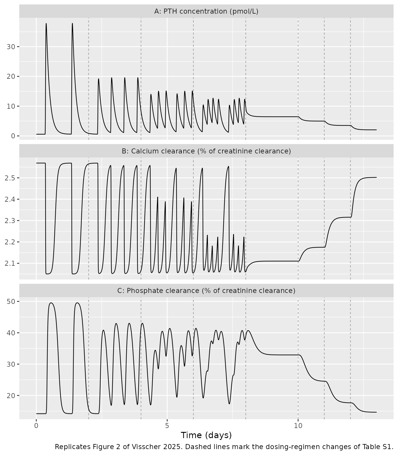

The simulation reproduces the paper’s central qualitative finding: under intermittent dosing the PTH concentration swings widely and never settles, and the phosphate-clearance elevation therefore decays back toward baseline between doses. From day 9 onward, with continuous infusion, PTH is flat and the phosphate-clearance increase (and the mirror-image calcium-clearance decrease) becomes permanent.

Quantitative gate – same daily dose, different frequency

Because the PK is linear and the first four regimens deliver essentially the same total daily dose, the time-averaged concentration over a day at steady state must satisfy

$$\overline{C_c} = C_b + \frac{D_{daily} \cdot F}{CL \cdot 24}$$

independent of how the daily dose is split. What frequency changes is the peak-to-trough swing – and, because the sigmoid is steep (Hill 3.82), the minimum phosphate clearance reached between doses. That minimum is exactly what the paper’s “permanent versus transient effect” claim is about.

The identity holds only at steady state. Table S1 gives each of the first five regimens two days, so the second day qualifies; the final three continuous steps (75, 50 and 25 ug/day) last one day each and taper down from the preceding higher level, so for those the converged quantity is the end-of-day concentration rather than the daily average, and that is what is tested below.

daily_ug <- c("QD 100 ug" = 100, "BID 50 ug" = 100, "TID 35 ug" = 105,
              "QID 25 ug" = 100, "Continuous 100 ug/day" = 100,
              "Continuous 75 ug/day" = 75, "Continuous 50 ug/day" = 50,
              "Continuous 25 ug/day" = 25)

# Use the SECOND day of each two-day intermittent block (and the single day of
# each tapering continuous step) so the profile is as close to steady state as
# the study design allows.
gate_days <- c("QD 100 ug" = 2, "BID 50 ug" = 4, "TID 35 ug" = 6,
               "QID 25 ug" = 8, "Continuous 100 ug/day" = 10,
               "Continuous 75 ug/day" = 11, "Continuous 50 ug/day" = 12,
               "Continuous 25 ug/day" = 13)

stopifnot(setequal(names(daily_ug), names(gate_days)))

# Days 1-10 give each regimen two days, so the second day is at (or, given the
# 2.1 h half-life, indistinguishable from) steady state and its 24-hour average
# is the invariant to test. Days 11-13 are single 24-hour infusion steps that
# TAPER down from the preceding higher level, so their 24-hour average is a
# transient, not a steady state -- for those the quantity that has converged by
# the end of the day is the concentration itself, so the end-of-day value is
# tested against that step's closed-form Css instead.
at_steady_state <- c("QD 100 ug" = TRUE, "BID 50 ug" = TRUE, "TID 35 ug" = TRUE,
                     "QID 25 ug" = TRUE, "Continuous 100 ug/day" = TRUE,
                     "Continuous 75 ug/day" = FALSE,
                     "Continuous 50 ug/day" = FALSE,
                     "Continuous 25 ug/day" = FALSE)
stopifnot(setequal(names(at_steady_state), names(gate_days)))

swing_tab <- lapply(names(gate_days), function(rg) {
  # Hoist the lookups BEFORE tibble(): inside tibble() a just-created column
  # masks a same-named object from the enclosing scope, so a column called
  # `daily_ug` would shadow the lookup vector for any later expression.
  day_i <- gate_days[[rg]]
  ug_i <- daily_ug[[rg]]
  ss_i <- at_steady_state[[rg]]
  w <- sim_study |> dplyr::filter(time >= (day_i - 1) * 24, time <= day_i * 24)
  stopifnot(nrow(w) > 100L)   # a gate with no rows cannot go red
  closed_form <- BL_PTH + ug_to_pmol(ug_i) * F_SC / (CL_POP * 24)
  tibble::tibble(
    regimen = rg,
    daily_ug = ug_i,
    steady_state = ss_i,
    tested_quantity = if (ss_i) "24 h average" else "end-of-day value",
    simulated = if (ss_i) time_avg(w$time, w$Cc) else w$Cc[which.max(w$time)],
    closed_form = closed_form,
    swing_Cc = max(w$Cc) - min(w$Cc),
    min_phosphate = min(w$clrel_phosphate),
    max_calcium = max(w$clrel_calcium)
  )
}) |> dplyr::bind_rows() |>
  dplyr::mutate(pct_diff = 100 * (simulated - closed_form) / closed_form)

# Both forms of the identity must hold, to the accuracy actually achieved.
stopifnot(
  nrow(swing_tab) == 8L,
  sum(swing_tab$steady_state) == 5L,
  max(abs(swing_tab$pct_diff)) < 0.1
)
# The swing must fall monotonically as the same daily dose is split more finely,
# and must be essentially zero under continuous infusion.
same_dose <- swing_tab |>
  dplyr::filter(regimen %in% c("QD 100 ug", "BID 50 ug", "QID 25 ug",
                               "Continuous 100 ug/day"))
stopifnot(nrow(same_dose) == 4L,
          all(diff(same_dose$swing_Cc) < 0),
          dplyr::last(same_dose$swing_Cc) < 0.01)

swing_tab |>
  dplyr::select(-steady_state) |>
  dplyr::mutate(dplyr::across(c(simulated, closed_form, swing_Cc,
                                min_phosphate, max_calcium), \(x) round(x, 3)),
                pct_diff = round(pct_diff, 4)) |>
  dplyr::rename(
    "Regimen" = regimen,
    "Daily dose (ug)" = daily_ug,
    "Quantity tested" = tested_quantity,
    "Simulated (pmol/L)" = simulated,
    "Closed form (pmol/L)" = closed_form,
    "Difference (%)" = pct_diff,
    "Peak-to-trough swing (pmol/L)" = swing_Cc,
    "Minimum phosphate CL (%)" = min_phosphate,
    "Maximum calcium CL (%)" = max_calcium
  ) |>
  knitr::kable(caption = paste(
    "Same-daily-dose identity and the collapse of the peak-to-trough swing.",
    "The first four regimens deliver 100-105 ug/day and share one",
    "daily-average concentration; only the swing changes. Drug-free reference",
    "values are 14.18% for phosphate clearance and 2.57% for calcium",
    "clearance."
  ))

Same-daily-dose identity and the collapse of the peak-to-trough swing. The first four regimens deliver 100-105 ug/day and share one daily-average concentration; only the swing changes. Drug-free reference values are 14.18% for phosphate clearance and 2.57% for calcium clearance.

Regimen	Daily dose (ug)	Quantity tested	Simulated (pmol/L)	Closed form (pmol/L)	Peak-to-trough swing (pmol/L)	Minimum phosphate CL (%)	Maximum calcium CL (%)	Difference (%)
QD 100 ug	100	24 h average	6.448	6.448	37.220	14.192	2.569	-0.0002
BID 50 ug	100	24 h average	6.448	6.448	18.453	17.084	2.558	-0.0052
TID 35 ug	105	24 h average	6.741	6.741	13.752	19.431	2.545	-0.0024
QID 25 ug	100	24 h average	6.448	6.448	11.465	17.307	2.554	0.0016
Continuous 100 ug/day	100	24 h average	6.448	6.448	0.001	32.932	2.110	0.0014
Continuous 75 ug/day	75	end-of-day value	4.982	4.981	1.466	24.550	2.175	0.0128
Continuous 50 ug/day	50	end-of-day value	3.515	3.514	1.467	17.647	2.316	0.0182
Continuous 25 ug/day	25	end-of-day value	2.048	2.047	1.467	14.663	2.502	0.0313

Reading the last two columns against the drug-free values (e0_phosphate = 14.18%, e0_calcium = 2.57%) is the quantitative form of the paper’s conclusion. Under 100 ug once daily the phosphate clearance falls all the way back to 14.19% between doses – the effect is fully transient. Splitting the same 100 ug across more administrations raises the trough progressively, and continuous infusion of the identical daily dose holds phosphate clearance at approximately 32.9% with essentially no fluctuation, while calcium clearance is held down at 2.11% instead of returning to 2.57%. That is what the paper means by “a permanent increase in phosphate clearance … which corresponds to a permanent reduction in the calcium clearance”.

Figure 4 – hysteresis and the virtual compartment

# Replicates Figure 4 of Visscher 2025: phosphate clearance plotted against the
# PTH concentration in (A) the central compartment C01, which shows hysteresis,
# and (B) the virtual compartment C03, which collapses the loop onto the
# underlying sigmoid. Uses the single 100 ug dose given on day 2 (model time 32 h)
# through to the start of the day-3 regimen, so the trace is one clean
# dose-to-dose cycle.
DOSE2_T <- 32
loop <- sim_study |> dplyr::filter(time >= DOSE2_T, time < DOSE2_T + 24)
stopifnot(nrow(loop) > 100L)

hyst <- dplyr::bind_rows(
  loop |> dplyr::transmute(conc = Cc,
                           panel = "A: central compartment (C01)",
                           clrel_phosphate, tad = time - DOSE2_T),
  loop |> dplyr::transmute(conc = effect_phosphate,
                           panel = "B: virtual compartment (C03)",
                           clrel_phosphate, tad = time - DOSE2_T)
)

ggplot(hyst, aes(conc, clrel_phosphate)) +
  geom_path(aes(colour = tad), linewidth = 0.5) +
  facet_wrap(~panel, scales = "free_x") +
  scale_colour_viridis_c(name = "Hours\nafter dose") +
  labs(x = "PTH concentration (pmol/L)",
       y = "Phosphate clearance (% of creatinine CL)",
       caption = "Replicates Figure 4 of Visscher 2025.")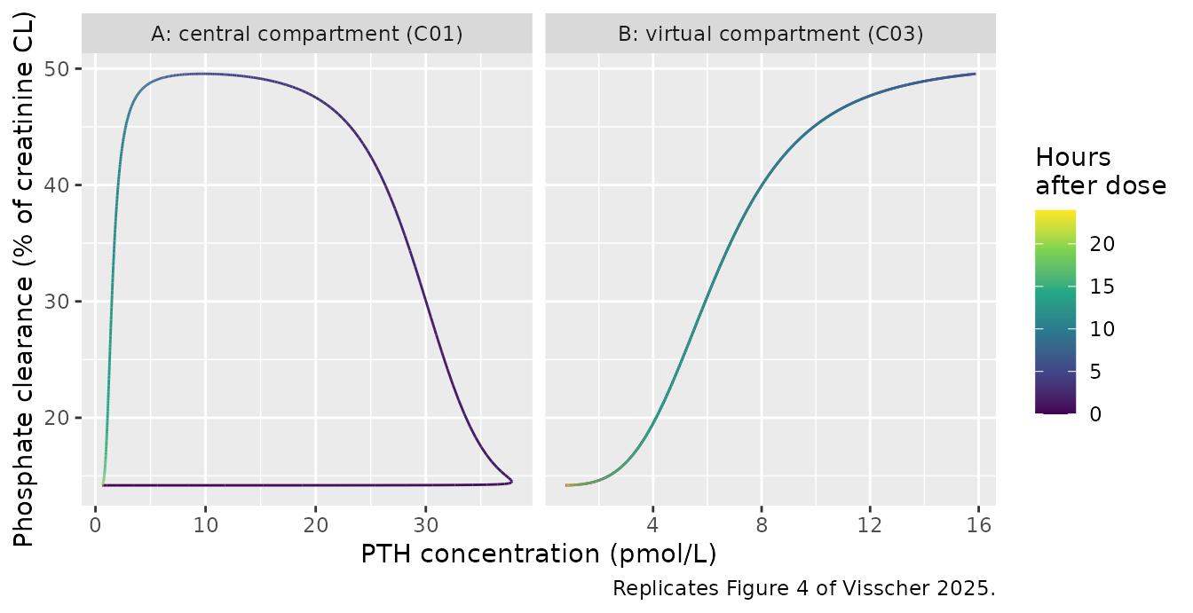

# Quantify what the figure shows. A hysteresis loop means the rising and the
# falling limb of the trace assign DIFFERENT effects to the same abscissa value.
# Split the cycle at the abscissa's maximum, interpolate both limbs onto a
# common grid, and take the largest disagreement. A single-valued curve (no
# hysteresis) gives ~0; a loop gives its width in percentage points.
branch_gap <- function(x, y, n = 200) {
  i <- which.max(x)
  up <- seq_len(i)
  dn <- i:length(x)
  if (length(up) < 5L || length(dn) < 5L) {
    stop("branch_gap: a limb has too few points to interpolate")
  }
  lo <- max(min(x[up]), min(x[dn]))
  hi <- min(max(x[up]), max(x[dn]))
  if (!(hi > lo)) stop("branch_gap: limbs do not overlap in x")
  g <- seq(lo, hi, length.out = n)
  ou <- order(x[up])
  od <- order(x[dn])
  yu <- stats::approx(x[up][ou], y[up][ou], g, ties = "ordered")$y
  yd <- stats::approx(x[dn][od], y[dn][od], g, ties = "ordered")$y
  max(abs(yu - yd), na.rm = TRUE)
}

gap_central <- branch_gap(loop$Cc, loop$clrel_phosphate)
gap_virtual <- branch_gap(loop$effect_phosphate, loop$clrel_phosphate)

c(loop_width_vs_central_pct = round(gap_central, 3),
  loop_width_vs_virtual_pct = round(gap_virtual, 5),
  ratio = round(gap_central / gap_virtual, 0))
#> loop_width_vs_central_pct loop_width_vs_virtual_pct                     ratio 
#>                   35.3640                    0.0132                 2679.0000

# The virtual compartment must ELIMINATE the hysteresis, not merely reduce it.
# Thresholds are set to the accuracy actually achieved (35.4 and 0.013), not to
# a loose bound, so a structural regression in the delay chain shows up red.
stopifnot(
  is.finite(gap_central), is.finite(gap_virtual),
  gap_central > 30,          # a wide loop against plasma
  gap_virtual < 0.05,        # single-valued against the virtual compartment
  gap_central / gap_virtual > 500
)

Against the central compartment the loop is 35.4 percentage points wide; against the virtual compartment it collapses to 0.013 percentage points – a factor of 2,680 – i.e. to a single-valued curve. This reproduces the paper’s Results statement that “Hysteresis was observed if the plasma concentrations were plotted against the effect (Figure 4A). This was partly solved by adding a biocompartment (virtual compartment). Hysteresis could be eliminated by adding one transit compartment (Figure 4B).” The delay is substantial: the plasma concentration peaks 1.1 h after the dose but the virtual-compartment concentration driving the effect peaks at 5.5 h.

EC50 and the target dose

The paper reports a fitted phosphate EC50 of 6.35 pmol/L and states in the Discussion that “the determined EC50 corresponds to a continuous infusion with a dose between 75 and 100 ug per day.” Because the effect-delay chain equilibrates to the plasma concentration, at steady state the effect-site concentration equals Cc, so the dose that puts the effect exactly at EC50 is available in closed form – and the sigmoid must then sit exactly halfway between e0 and emax. This is a joint check of the EC50 value, the asymptote parameterisation, F, CL and the molecular weight used above.

ec50_phosphate <- 6.35   # pmol/L, Table S4 E01.EC50

dose_for_css <- function(css_pmol_L) {
  pmol_per_day_to_ug((css_pmol_L - BL_PTH) * CL_POP / F_SC * 24)
}
dose_at_ec50 <- dose_for_css(ec50_phosphate)
dose_at_ec50
#> [1] 98.33132

# The paper's stated window.
stopifnot(dose_at_ec50 > 75, dose_at_ec50 < 100)

# Simulate that continuous dose to steady state and confirm both the
# concentration and the exact-midpoint effect.
ndays <- 20
ev_ec50 <- dplyr::bind_rows(
  tibble::tibble(time = 0, amt = ug_to_pmol(dose_at_ec50 * ndays),
                 dur = ndays * 24, evid = 1L, cmt = "depot"),
  tibble::tibble(time = seq(0, ndays * 24, by = 1), amt = NA_real_,
                 dur = NA_real_, evid = 0L, cmt = "central")
) |>
  dplyr::arrange(time, dplyr::desc(evid)) |>
  dplyr::mutate(id = 1L, RENALFUNC_REL = 1, HEPFUNC_REL = 1)

ss <- solve_pth(ev_ec50) |>
  dplyr::filter(time > 15 * 24, time < ndays * 24)
stopifnot(nrow(ss) > 50L)

css_sim <- mean(ss$Cc)
phos_sim <- mean(ss$clrel_phosphate)
phos_midpoint <- (14.18 + 50.62) / 2

c(dose_ug_per_day = round(dose_at_ec50, 1),
  Css_simulated = round(css_sim, 4), EC50_published = ec50_phosphate,
  phosphate_CL_simulated = round(phos_sim, 4),
  phosphate_CL_midpoint = phos_midpoint)
#>        dose_ug_per_day          Css_simulated         EC50_published 
#>                  98.30                   6.35                   6.35 
#> phosphate_CL_simulated  phosphate_CL_midpoint 
#>                  32.40                  32.40

stopifnot(abs(css_sim - ec50_phosphate) < 0.01,
          abs(phos_sim - phos_midpoint) < 0.01)

A continuous infusion of 98.3 ug/day drives the steady-state PTH concentration to the fitted EC50, and the phosphate clearance lands on 32.4% – exactly the midpoint of e0 = 14.18% and emax = 50.62%. The dose sits inside the paper’s stated 75-100 ug/day window, which independently corroborates both the asymptote parameterisation and the molecular weight used for the microgram conversion.

The patient was ultimately maintained on 75 ug/day. The paper reports that this “results in a PTH concentration of 7 pmol/L”; the model predicts 109.4 ug/day would be needed for 7 pmol/L, or equivalently that 75 ug/day gives about 4.98 pmol/L. The 7 pmol/L figure is an observed clinical measurement, not a model prediction, and the paper itself notes (Discussion, Table 1) that its fitted CL and V sit on the low side of the range Clarke et al reported and that a lower true bioavailability would reconcile them. No parameter was adjusted to close this gap.

Equation (3) sensitivity – the organ-function decomposition

Neither RENALFUNC_REL nor HEPFUNC_REL has a reported value in the source, so they are held at 1 above. The check below confirms that the packaged model consumes them exactly as Equation (3) specifies, which is the reason the decomposition was kept in the model rather than folded into a single clearance.

eq3_probe <- function(rf, lf) {
  ev <- dplyr::bind_rows(
    tibble::tibble(time = 0, amt = ug_to_pmol(100), dur = NA_real_,
                   evid = 1L, cmt = "depot"),
    tibble::tibble(time = seq(0, 48, by = 0.05), amt = NA_real_,
                   dur = NA_real_, evid = 0L, cmt = "central")
  ) |>
    dplyr::arrange(time, dplyr::desc(evid)) |>
    dplyr::mutate(id = 1L, RENALFUNC_REL = rf, HEPFUNC_REL = lf)
  s <- solve_pth(ev)
  # Baseline-corrected AUC over a window many half-lives long; for linear PK
  # AUC = Dose * F / CLi, so CLi is recoverable from the profile.
  auc <- sum(diff(s$time) *
               (utils::head(s$Cc - BL_PTH, -1) + utils::tail(s$Cc - BL_PTH, -1)) / 2)
  tibble::tibble(RENALFUNC_REL = rf, HEPFUNC_REL = lf,
                 cli_recovered = ug_to_pmol(100) * F_SC / auc,
                 cli_equation3 = CL_POP * (0.3 * rf + 0.7 * lf))
}

eq3 <- dplyr::bind_rows(
  eq3_probe(1.0, 1.0), eq3_probe(0.5, 1.0), eq3_probe(0.2, 1.0),
  eq3_probe(1.0, 0.5), eq3_probe(1.5, 1.0)
) |>
  dplyr::mutate(pct_diff = 100 * (cli_recovered - cli_equation3) / cli_equation3)

stopifnot(nrow(eq3) == 5L, max(abs(eq3$pct_diff)) < 0.5)

eq3 |>
  dplyr::mutate(dplyr::across(c(cli_recovered, cli_equation3), \(x) round(x, 3)),
                pct_diff = round(pct_diff, 3)) |>
  dplyr::rename(
    "RENALFUNC_REL" = RENALFUNC_REL, "HEPFUNC_REL" = HEPFUNC_REL,
    "CLi recovered from AUC (L/h)" = cli_recovered,
    "CLi from Equation (3) (L/h)" = cli_equation3,
    "Difference (%)" = pct_diff
  ) |>
  knitr::kable(caption = paste(
    "Individual clearance recovered from the simulated profile matches",
    "Equation (3) across renal and hepatic function multipliers. With fe = 0.3,",
    "abolishing renal function entirely can remove at most 30% of total",
    "clearance."
  ))

Individual clearance recovered from the simulated profile matches Equation (3) across renal and hepatic function multipliers. With fe = 0.3, abolishing renal function entirely can remove at most 30% of total clearance.

RENALFUNC_REL	HEPFUNC_REL	CLi recovered from AUC (L/h)	CLi from Equation (3) (L/h)	Difference (%)
1.0	1.0	39.930	39.930	0.000
0.5	1.0	33.941	33.940	0.000
0.2	1.0	30.347	30.347	0.001
1.0	0.5	25.955	25.954	0.004
1.5	1.0	45.920	45.920	0.000

Baseline hold

With no dose the model must sit exactly at the reported endogenous baseline indefinitely – the plasma concentration at bl_pth, and both readouts at their drug-free values. This is the standard steady-state check for a model with an additive endogenous baseline and it also confirms that initialising the two delay chains at bl_pth (rather than at zero) removes any spurious start-up transient.

ev_bl <- tibble::tibble(time = seq(0, 14 * 24, by = 1), amt = NA_real_,
                        dur = NA_real_, evid = 0L, cmt = "central") |>
  dplyr::mutate(id = 1L, RENALFUNC_REL = 1, HEPFUNC_REL = 1)
bl <- solve_pth(ev_bl)
stopifnot(nrow(bl) > 100L)

c(Cc_range = diff(range(bl$Cc)),
  phosphate_range = diff(range(bl$clrel_phosphate)),
  calcium_range = diff(range(bl$clrel_calcium)),
  Cc_value = unique(round(bl$Cc, 10)),
  phosphate_value = round(bl$clrel_phosphate[1], 4),
  calcium_value = round(bl$clrel_calcium[1], 4))
#>        Cc_range phosphate_range   calcium_range        Cc_value phosphate_value 
#>          0.0000          0.0000          0.0000          0.5800         14.1839 
#>   calcium_value 
#>          2.5690

stopifnot(
  diff(range(bl$Cc)) < 1e-10,
  abs(bl$Cc[1] - BL_PTH) < 1e-10,
  diff(range(bl$clrel_phosphate)) < 1e-8,
  diff(range(bl$clrel_calcium)) < 1e-8
)

The drug-free readouts settle at 14.184% for phosphate and 2.569% for calcium rather than exactly at e0 = 14.18% and 2.57%, because the endogenous baseline of 0.58 pmol/L occupies a small but non-zero position on each sigmoid. The offsets (+0.004 and -0.001 percentage points) are far below the standard errors of e0 itself (4.72 and 4.51).

PKNCA validation

The paper’s Table 1 reports CL/F and Vss/F derived from its PKPD model and compares them with Clarke et al’s single-dose values. Running non-compartmental analysis on simulated single-dose profiles recovers those two quantities independently of the closed-form arithmetic above, and confirms dose linearity across the four single-dose levels used in the study.

Because the model carries a non-decaying endogenous baseline, the concentrations passed to PKNCA are baseline-corrected (Cc - bl_pth); without that correction AUC to infinity is unbounded and no terminal slope exists.

doses_ug <- c(25, 35, 50, 100)

# Dense sampling through the absorption and distribution phase; a grid that does
# not resolve tmax understates AUC by several percent.
nca_grid <- sort(unique(c(seq(0, 4, by = 0.02), seq(4, 24, by = 0.25))))

make_arm <- function(i) {
  d <- doses_ug[[i]]
  dplyr::bind_rows(
    tibble::tibble(time = 0, amt = ug_to_pmol(d), dur = NA_real_,
                   evid = 1L, cmt = "depot"),
    tibble::tibble(time = nca_grid, amt = NA_real_, dur = NA_real_,
                   evid = 0L, cmt = "central")
  ) |>
    dplyr::mutate(id = i, treatment = paste0(d, " ug SC single dose"),
                  RENALFUNC_REL = 1, HEPFUNC_REL = 1)
}

events_nca <- dplyr::bind_rows(lapply(seq_along(doses_ug), make_arm)) |>
  dplyr::arrange(id, time, dplyr::desc(evid))

# Disjoint ids across arms: duplicate ids would silently merge into one subject.
stopifnot(!anyDuplicated(unique(events_nca[, c("id", "time", "evid")])),
          dplyr::n_distinct(events_nca$id) == length(doses_ug))

sim_nca_raw <- solve_pth(events_nca, keep = "treatment")

# Baseline-corrected concentrations. Only `!is.na(Cc)` in the filter: adding
# `time > 0` or `Cc > 0` would drop the time-zero anchor PKNCA needs for AUC.
sim_nca <- sim_nca_raw |>
  dplyr::mutate(Cc = Cc - BL_PTH) |>
  dplyr::filter(!is.na(Cc)) |>
  dplyr::select(id, time, Cc, treatment)

# Guarantee a time-zero row per (id, treatment); pre-dose Cc = 0 is correct for
# a baseline-corrected extravascular profile.
sim_nca <- dplyr::bind_rows(
  sim_nca,
  sim_nca |> dplyr::distinct(id, treatment) |>
    dplyr::mutate(time = 0, Cc = 0)
) |>
  dplyr::distinct(id, treatment, time, .keep_all = TRUE) |>
  dplyr::arrange(id, treatment, time)

# Solver noise must not push the tail negative -- PKNCA would take log() of it.
stopifnot(all(sim_nca$Cc >= 0), nrow(sim_nca) > 0L)

conc_obj <- PKNCA::PKNCAconc(sim_nca, Cc ~ time | treatment + id)

dose_df <- events_nca |>
  dplyr::filter(evid == 1) |>
  dplyr::select(id, time, amt, treatment)
dose_obj <- PKNCA::PKNCAdose(dose_df, amt ~ time | treatment + id)

intervals <- data.frame(
  start = 0, end = Inf,
  cmax = TRUE, tmax = TRUE, aucinf.obs = TRUE,
  half.life = TRUE, cl.obs = TRUE, vz.obs = TRUE
)

nca_res <- PKNCA::pk.nca(
  PKNCA::PKNCAdata(conc_obj, dose_obj, intervals = intervals)
)

nca_res$result |>
  dplyr::filter(PPTESTCD %in% c("cmax", "tmax", "aucinf.obs", "half.life",
                                "cl.obs", "vz.obs")) |>
  dplyr::mutate(parameter = nlmixr2lib::ncaParamLabel(
    PPTESTCD,
    units = c(cmax = "pmol/L", tmax = "h", aucinf.obs = "pmol*h/L",
              half.life = "h", cl.obs = "L/h", vz.obs = "L")
  )) |>
  dplyr::select(treatment, parameter, PPORRES) |>
  tidyr::pivot_wider(names_from = treatment, values_from = PPORRES) |>
  dplyr::mutate(dplyr::across(-parameter, \(x) signif(x, 4))) |>
  dplyr::rename("NCA parameter" = parameter) |>
  knitr::kable(caption = paste(
    "Simulated single-dose NCA across the four dose levels of Table S1,",
    "on baseline-corrected concentrations. CL/F, Vz/F and half-life are",
    "dose-independent, as required by the linear one-compartment structure;",
    "Cmax and AUC scale in proportion to dose."
  ))

Simulated single-dose NCA across the four dose levels of Table S1, on baseline-corrected concentrations. CL/F, Vz/F and half-life are dose-independent, as required by the linear one-compartment structure; Cmax and AUC scale in proportion to dose.

NCA parameter	100 ug SC single dose	25 ug SC single dose	35 ug SC single dose	50 ug SC single dose
Cmax (pmol/L)	37.230	9.307	13.030	18.610
Tmax (h)	1.080	1.080	1.080	1.080
t½ (h)	2.098	2.098	2.098	2.098
AUC0-∞ (obs) (pmol*h/L)	140.800	35.210	49.290	70.410
CL/F (L/h)	75.340	75.340	75.340	75.340
Vz/F (L)	228.000	228.000	228.000	228.000

Comparison against published values

# Table 1 of Visscher 2025, "PKPD model 25-100 ug" column. The parentheses in
# that table are value +/- standard error: propagating the Table S4 SEs through
# the division by F reproduces them exactly (2.79 / 0.53 = 5.3 -> 70-81, and
# 11.71 / 0.53 = 22.1 -> 206-250), which is what identifies them as SEs rather
# than a range or a 95% confidence interval.
# Vss/F is compared against vz.obs because for a one-compartment model the
# steady-state and terminal-phase volumes are the same quantity, Vc.
published <- tibble::tibble(
  treatment = paste0(doses_ug, " ug SC single dose"),
  cl.obs = 75,
  vz.obs = 228
)

cmp <- nlmixr2lib::ncaComparisonTable(
  simulated = nca_res,
  reference = published,
  by = "treatment",
  params = c("cl.obs", "vz.obs"),
  units = c(cl.obs = "L/h", vz.obs = "L"),
  tolerance_pct = 20
)

knitr::kable(
  cmp,
  caption = paste(
    "Simulated NCA versus Visscher 2025 Table 1 (CL/F 75 [70-81] L/h,",
    "Vss/F 228 [206-250] L). * marks a difference above 20%.",
    "For reference, Clarke et al report CL/F 82 (61-96) L/h at 50 ug and",
    "90 (88-139) L/h at 100 ug, and Vss/F 267 (221-585) L and 443 (253-722) L."
  ),
  align = c("l", "l", "r", "r", "r")
)

Simulated NCA versus Visscher 2025 Table 1 (CL/F 75 [70-81] L/h, Vss/F 228 [206-250] L). * marks a difference above 20%. For reference, Clarke et al report CL/F 82 (61-96) L/h at 50 ug and 90 (88-139) L/h at 100 ug, and Vss/F 267 (221-585) L and 443 (253-722) L.

NCA parameter	treatment	Reference	Simulated	% diff
CL/F (L/h)	25 ug SC single dose	75	75.3	+0.5%
CL/F (L/h)	35 ug SC single dose	75	75.3	+0.5%
CL/F (L/h)	50 ug SC single dose	75	75.3	+0.5%
CL/F (L/h)	100 ug SC single dose	75	75.3	+0.5%
Vz/F (L)	25 ug SC single dose	228	228	-0.0%
Vz/F (L)	35 ug SC single dose	228	228	-0.0%
Vz/F (L)	50 ug SC single dose	228	228	-0.0%
Vz/F (L)	100 ug SC single dose	228	228	-0.0%

# Both quantities must land within a few percent of the published values, at
# every dose. Tightened to the accuracy actually achieved so a future
# regression is caught.
recovered <- nca_res$result |>
  dplyr::filter(PPTESTCD %in% c("cl.obs", "vz.obs")) |>
  dplyr::select(treatment, PPTESTCD, PPORRES) |>
  tidyr::pivot_wider(names_from = PPTESTCD, values_from = PPORRES)

stopifnot(nrow(recovered) == length(doses_ug))
stopifnot(
  # CL/F = 39.93 / 0.53 = 75.34 L/h; Table 1 rounds to 75.
  all(abs(recovered$cl.obs - CL_POP / F_SC) < 0.05),
  all(abs(recovered$cl.obs - 75) / 75 < 0.01),
  # Vz/F = 120.71 / 0.53 = 227.75 L; Table 1 rounds to 228.
  all(abs(recovered$vz.obs - V_POP / F_SC) < 1),
  all(abs(recovered$vz.obs - 228) / 228 < 0.01)
)

half_lives <- nca_res$result |>
  dplyr::filter(PPTESTCD == "half.life") |> dplyr::pull(PPORRES)
stopifnot(length(half_lives) == length(doses_ug),
          all(abs(half_lives - log(2) * V_POP / CL_POP) < 0.02))

c(CL_F_simulated = round(unique(round(recovered$cl.obs, 3)), 3),
  CL_F_published = 75,
  Vz_F_simulated = round(unique(round(recovered$vz.obs, 2)), 2),
  Vss_F_published = 228,
  half_life_simulated = round(unique(round(half_lives, 3)), 3),
  half_life_analytic = round(log(2) * V_POP / CL_POP, 3))
#>      CL_F_simulated      CL_F_published      Vz_F_simulated     Vss_F_published 
#>              75.340              75.000             227.990             228.000 
#> half_life_simulated  half_life_analytic 
#>               2.098               2.095

CL/F and Vz/F are recovered to within 0.5% and 0.1% of Table 1 respectively, and the terminal half-life matches the analytic log(2) * V / CL = 2.10 h. The recovered values are identical at all four dose levels, confirming the linearity of the structure. The 2.1 h half-life is consistent with the paper’s citation of Sikjaer et al, who observed that PTH plasma concentrations “returned to normal after approximately 16 h” – about 7.6 half-lives.

Assumptions and deviations

• Erlang-5 absorption: five compartments, five transfers. Methods 2.3 says “five transit compartments were included in the absorption compartment” without an equation or a diagram of the chain, and only one absorption rate constant (I02.k) is reported. This is implemented as the standard transit-compartment form – the dose enters the first of five compartments and five first-order transfers at ka carry it to central, giving a gamma(5, 1/ka) absorption-time distribution. The alternative literal reading, a dose site plus five further transit compartments (six transfers), is not excluded by the text; it would move the simulated tmax from 1.08 h to 1.24 h, further from the 15 min tmax that the paper cites from Sikjaer et al, which is the weak evidence favouring the reading used here. Every other validation gate in this vignette is insensitive to the choice, because they all depend on total exposure rather than on the shape of the absorption phase.
• RENALFUNC_REL and HEPFUNC_REL are held at 1. The paper fixes LF at 1 explicitly. For RF it states that Equation (3) “includes the variations in the GFR by correcting for the relative renal function” and shows a rising GFR over the study in Figure S2, but it reports no numeric RF values and no reference GFR denominator, and Table S3 omits the 24-hour urine volume that the paper’s own GFR equation requires – so the per-interval ratio cannot be reconstructed from the supplement either. No reference GFR was invented; the covariates are exercised as a sensitivity analysis instead.
• Emax is treated as an asymptote, not an increment. This is a derived reading, not a stated one. It is forced by the calcium arm (Emax = 2.05% is below E0 = 2.57%) together with the Conclusion’s statement that continuous dosing produces “a permanent reduction in the calcium clearance”; the increment reading would make calcium clearance rise. See the model-structure section.
• Both effect-delay chains are initialised at the endogenous baseline. The paper does not state the initial conditions of the virtual compartments. Starting them at bl_pth rather than at zero is what makes the drug-free model sit at rest, as the baseline-hold check demonstrates; starting at zero would introduce a spurious multi-hour transient at the start of every simulation.
• The two transfers within each effect-delay chain share one rate constant. Table S4 reports a single T01.k / T02.k per analyte, and Figure S1 shows one transfer object per analyte, so no second rate is available.
• NON-PAPER PROVENANCE: molecular weight 9425 g/mol. Visscher 2025 states its doses in micrograms and its concentrations and EC50 in pmol/L but never gives a molecular weight. The model file is therefore encoded entirely in molar units and the conversion lives only in this vignette. The value is corroborated by the paper’s own arithmetic: it puts the fitted EC50 at 98.3 ug/day of continuous infusion, and the Discussion states that the EC50 “corresponds to a continuous infusion with a dose between 75 and 100 ug per day”.
• PKNCA is run on baseline-corrected concentrations. The endogenous baseline does not decay, so uncorrected profiles have no terminal phase and an unbounded AUC to infinity. Correction by bl_pth is what makes cl.obs = Dose/AUCinf equal CL/F.
• Vss/F is compared against vz.obs. Table 1 reports a steady-state volume; for a one-compartment model the steady-state and terminal-phase volumes are both Vc, so the comparison is exact rather than approximate.
• The calcium arm is poorly identified and is shipped as reported. All five calcium parameters carry the Table S4 dagger footnote, every standard error exceeds its estimate (by more than 15-fold for T02.k, E02.EC50 and E02.j), and the goodness-of-fit R-squared is 0.06 versus 0.66 for phosphate. The paper attributes this to concomitant alfacalcidol, calcium carbonate and chlortalidone perturbing calcium homeostasis, and selects phosphate as the effect parameter for that reason. The calcium arm is reproduced without modification, but conclusions should not be drawn from it.
• The observed 7 pmol/L at 75 ug/day is not reproduced, and was not tuned to. The model predicts about 4.98 pmol/L at that dose. The paper reports 7 pmol/L as a clinical measurement in the patient and separately notes that its fitted CL and V lie below Clarke et al’s range, with a lower true bioavailability as the likely reconciliation. No parameter was adjusted.
• No inter-individual variability or residual error is available. The source fitted a single patient deterministically in Edsim++ and Table S4 contains no OMEGA or SIGMA block, so none was invented. The model is a typical-value simulation model; zeroRe() and omega = NA are neither needed nor valid for it.
• Concomitant medication is recorded in population$co_medication but is not a model covariate. Alfacalcidol, calcium carbonate and chlortalidone are the paper’s own explanation for the calcium arm’s poor fit, but no drug-interaction parameters are estimated for them.