Aducanumab amyloid-beta QSP (Lin 2022)

Model and source

Lin and colleagues (Biogen and Applied BioMath) built a quantitative systems pharmacology (QSP) model of the amyloid-beta (A-beta) pathway in Alzheimer’s disease and of the mechanism of action of aducanumab, a human IgG1 antibody that binds aggregated A-beta. The model was calibrated to literature A-beta biology, single-ascending-dose (SAD) PK and plasma A-beta, and one year of amyloid-PET SUVR from the phase Ib PRIME study, then validated against multiple-dose PK, two-year SUVR and a dose-titration cohort.

mod <- readModelDb("Lin_2022_aducanumab_qsp")
ui <- rxode2::rxode(mod)

• Citation: Lin L, Hua F, Salinas C, Young C, Bussiere T, Apgar JF, Burke JM, Kandadi Muralidharan K, Rajagovindan R, Nestorov I. Quantitative systems pharmacology model for Alzheimer’s disease to predict the effect of aducanumab on brain amyloid. CPT Pharmacometrics Syst Pharmacol. 2022;11(3):362-372. doi:10.1002/psp4.12759. Reaction network, compartment volumes and parameter values from Supplementary Model Code (S2, KroneckerBio model file); parameter provenance and units from Table S2; pretreatment steady state from the Supplementary_Initial_Condition sheet (S3); equations from S4.
• Article: https://doi.org/10.1002/psp4.12759
• Supplementary material (Tables S1-S3, model code, initial conditions, equations): https://www.ebi.ac.uk/europepmc/webservices/rest/PMC8923729/supplementaryFiles

QSP. Amyloid-beta (A-beta) pathway and aducanumab mechanism-of-action model in early Alzheimer’s disease. Thirty-six mass-action ODE states in three physiologic compartments (plasma 3 L, CSF 0.139 L, brain interstitial fluid 0.261 L) plus a peripheral aducanumab compartment: APP synthesis and sequential beta-secretase (BACE) and gamma-secretase cleavage to A-beta monomer in plasma and brain ISF, shedding of soluble BACE, monomer-oligomer exchange in every compartment, oligomer-plaque exchange in brain ISF, inter-compartment transport of monomer, oligomer, soluble BACE, drug and soluble drug-A-beta complexes, two-compartment aducanumab disposition, drug binding to monomer, oligomer and plaque, and FcR-mediated antibody-dependent cellular phagocytosis (ADCP) that clears drug-oligomer and drug-plaque complexes in brain ISF. States are amounts in nmol; second-order rates divide by the volume of the compartment in which the reaction occurs. The primary PD output is the percent change in total brain plaque, which the paper equates with the percent change in amyloid-PET composite SUVR above a cutoff of 1.0. Deterministic: no between-subject variability or residual error is reported. Nominal (final) parameter set; the paper’s alternative faster-plaque-turnover set (Table S3) is reproduced in the vignette. The system is stiff and badly scaled (states span 1e-3 to 1.5e5 nmol): solve with tight tolerances, e.g. rxSolve(…, atol = 1e-14, rtol = 1e-10, maxsteps = 5e6); rxode2’s defaults fail.

The model is built as mass-action reactions between amounts (nmol). A zero-order synthesis is an amount rate, a first-order reaction acts on an amount, and a bimolecular reaction in a compartment of volume V runs at k * x1 * x2 / V. This is the convention of the KroneckerBio model file the authors deposited, and it can be checked directly against the published initial conditions: for example the APP-BACE complex in plasma sits at konPP * APP * BACE / V / (koffBACE + kcatBACE) = 1e-3 * 28.936 * 88.529 / 3 / 120 = 0.0071157 nmol, which is the published value to five digits.

Solver settings. Gamma-secretase sits at 150,000 nmol while the enzyme-substrate complexes are near 0.001 nmol, and several binding reactions equilibrate in milliseconds (the plasma oligomer dissociates at 1.4e5 /s). The solve is therefore stiff and badly scaled. rxode2’s default tolerances fail, and so do some intermediate settings (atol = 1e-12, rtol = 1e-10 fails at 0.3 mg/kg). The maintainers tested every simulation in this article at several tolerance pairs. atol = 1e-14, rtol = 1e-10, atol = 1e-13, rtol = 1e-10 and atol = 1e-14, rtol = 1e-12 each solved all of them, and gave the same results. The last of these emits step-size warnings on multi-decade horizons. The helper below uses the first pair and falls back to the other two. Use tolerances at least this tight for any simulation with this model.

solve <- function(model, events, ...) {
  tols <- list(c(1e-14, 1e-10), c(1e-13, 1e-10), c(1e-14, 1e-12))
  for (i in seq_along(tols)) {
    out <- tryCatch(
      rxode2::rxSolve(
        model, events, ...,
        atol = tols[[i]][1], rtol = tols[[i]][2], maxsteps = 5e6,
        returnType = "data.frame"
      ),
      error = function(e) if (i == length(tols)) stop(e) else NULL
    )
    if (!is.null(out)) {
      return(out)
    }
  }
}

Population

The model represents a typical patient with early Alzheimer’s disease rather than a fitted population. It was calibrated to group means (Table S1): baseline concentrations of A-beta monomer, oligomer and plaque in plasma, CSF and brain interstitial fluid (ISF) from the literature; SILK A-beta kinetics in CSF; serum aducanumab PK and plasma A-beta from the SAD study (0.3-60 mg/kg, mild to moderate AD); CSF aducanumab concentrations; and 1-year SUVR from the placebo-controlled period of PRIME (1-10 mg/kg every 4 weeks, prodromal or mild AD). The paper reports no subject counts or demographics. Doses are converted from mg/kg at a body weight of 70 kg, which the maintainers inferred from Figure 2a (below).

str(ui$population, give.attr = FALSE)
#> List of 7
#>  $ species      : chr "human"
#>  $ n_subjects   : int NA
#>  $ n_studies    : int 3
#>  $ disease_state: chr "Mild-to-moderate Alzheimer's disease (single-ascending-dose study) and prodromal or mild Alzheimer's disease wi"| __truncated__
#>  $ dose_range   : chr "Calibration: 0.3-60 mg/kg single i.v. dose (SAD) and 1-10 mg/kg i.v. q4w for 1 year (MAD placebo-controlled per"| __truncated__
#>  $ regions      : chr "Not reported (Biogen clinical program)"
#>  $ notes        : chr "QSP calibrated to group-mean data, not a population fit. Table S1 lists the calibration and validation data: li"| __truncated__

Source trace

Every ini() value in the model file carries a comment naming its source. The values are those of the deposited model code (Supplementary Model Code, % Parameters), which prints four or five significant figures; Table S2 prints three and gives the provenance (“Fitted”, a literature reference, or “assumed”). The rows where the two sources disagree, and how each was settled, are listed under Parameter conflicts below.

Element	Value used	Source
Plasma, CSF, brain ISF volumes	3, 0.139, 0.261 L	Model code, % Compartments
Reaction network (36 states, 65 reactions)	–	Model code, % Reactions; Equations in S4
APP synthesis (plasma, ISF), degradation	1.44405e-3, 2.5127e-4 nmol/s; 4.8135e-5 /s	Model code / Table S2; plasma rate from the S3 steady state
BACE synthesis (plasma, ISF), degradation, shedding	1.08306e-3, 1.0365e-4 nmol/s; 1.2034e-5, 2.0e-7 /s	Model code / Table S2; plasma rate from the S3 steady state
Soluble BACE clearance	6.4180e-5 /s	Model code / Table S2
Gamma-secretase synthesis (plasma, ISF), clearance	28.8811, 2.5127 nmol/s; 1.9254e-4 /s	Model code / Table S2
konPP, konPD, konPF	1e-3 /nM/s	Model code / Table S2
koffBACE, kcatBACE, koffGamma, kcatGamma	119.9928, 0.0072, 215.9983, 0.0017 /s	Model code / Table S2
A-beta clearance: monomer, oligomer (plasma); monomer, oligomer, plaque (ISF)	9.627e-5, 9.627e-5, 1.9254e-5, 2.204e-8, 4.408e-9 /s	Model code / Table S2
kM2G; kG2M plasma, CSF, ISF	1.4e-5; 1.4e5, 0.0028, 1.4e-8 /s	Model code (ISF value, see below)
kG2P, kP2G_bisf	7e-8, 7e-11 /s	Model code / Table S2
Transport plasma to/from CSF (all species)	1.7222e-9 / 4.1667e-5 /s	Model code / Table S2
Transport plasma to/from ISF: monomer, oligomer, sBACE, drug, drug-oligomer	1.4811e-4/1.4811e-5, 1.4811e-6/1.4811e-8, 2.0056e-8/8.0226e-5, 1.6045e-6/0.0032, 1.6045e-6/1.4811e-8 /s	Model code / Table S2
Transport ISF to CSF: monomer, oligomer, sBACE, drug, drug-oligomer	1.5509e-5, 2.3264e-8, 1.5509e-5, 1.5509e-5, 2.3264e-8 /s	Model code / Table S2
Aducanumab elimination, k12mAb, k21mAb	1.4586e-6, 2.5e-6, 1e-6 /s	Model code / Table S2
koffma0 (monomer)	10 /s	Model code (see below)
koffma1 (oligomer), koffma2 (plaque)	0.02 /s	Table S2 and text (see below)
FcR synthesis, degradation; koffPF; kcatADCP	5.0253e-5 nmol/s, 1.9254e-4 /s; 10 /s; 0.0036 /s	Model code / Table S2
Infusion	dose over 2 h into plasma	Table S2 (kinfusion); S4
Initial conditions (pretreatment steady state)	23 non-zero states	S3, Supplementary_Initial_Condition
% plaque reduction	100 (P(t) - P(0)) / P(0)	Methods, ‘SUVR data processing’
Aducanumab molar mass	150,000 g/mol	Not printed; back-solved from Figure 3a (below)
A-beta molar mass	4,330 g/mol	Not printed; back-solved from Figure 2b (below)

Parameter conflicts between the model code and Table S2

The deposited model code and Table S2 disagree on five values. Each was settled against a published output of the model rather than by preference for one document:

Parameter	Model code	Table S2	Used	Deciding evidence
ksynthAPP_plasma	0.0014	1.40e-3	1.44405e-3 nmol/s	S3 steady state
ksynthBACE_plasma	0.0011	1.10e-3	1.08306e-3 nmol/s	S3 steady state
kG2M_bisf	1.4000e-08	1.48e-08	1.40e-8 /s	S3 steady state
koffma0	10	1.00	10 /s	Figure 2b
koffma1, koffma2	0.0180	2.00e-2	0.02 /s	Figures 2c and 3a; text “20 nM”

• The two synthesis rates. The model code prints every value at or above 0.001 with four decimals, so 0.0014 and 0.0011 carry only two significant figures. Table S2 appears to transcribe that display. At steady state, APP synthesis must equal kclearAPP * APP + kcatBACE * APP_BACE and BACE synthesis must equal (kclearBACE + kcleave) * BACE. The published S3 state therefore fixes them at 1.44405e-3 and 1.08306e-3 nmol/s. With these two values the S3 state is a steady state of the model (checked below); with the printed 0.0014 every A-beta species drifts by about 1.2%, and plasma A-beta settles at 493 rather than the 500 pg/mL baseline drawn in Figure 2b.
• kG2M_bisf. With the code value 1.40e-8, every A-beta species in the S3 state is uniformly consistent. With the Table S2 value 1.48e-8 the ISF oligomer and plaque states drift away from the rest.
• koffma0. Monomer binding is what raises total plasma A-beta after a 60 mg/kg dose (Figure 2b). With the code value 10 /s the model reproduces the published curve; with 1 /s the simulated peak is about 4,600 pg/mL against a published peak of about 1,300.
• koffma1, koffma2. The text states that the drug-plaque affinity “was estimated to be 20 nM” (0.02 / 1e-3), matching Table S2. The code prints 0.0180. The 1-year and 2-year plaque curves of Figures 2c and 3a are reproduced with 0.02 (root-mean-square error 0.3 percentage points against the digitised curves), and are systematically overpredicted with 0.018 (error 2.8 points). Table S2 assumes the oligomer affinity equals the plaque affinity, so both are set to 0.02.

Pretreatment steady state

The model starts from the published pretreatment steady state (S3). The paper states that plaque had reached steady state before treatment (Results, ‘Model calibration’), so the untreated model should not move. The check below runs it for 1000 years. States that S3 prints with only three significant figures near 1e-11 nmol are excluded from the relative comparison.

ss <- solve(ui, rxode2::et(c(0, 1000 * 365.25)))
states <- ui$state
start <- unlist(ss[1, states])
end <- unlist(ss[2, states])
big <- abs(start) > 1e-6
drift <- abs(end[big] - start[big]) / abs(start[big])
signif(max(drift), 3)
#> [1] 9.86e-05
stopifnot(max(drift) < 2e-4)

baseline <- tibble::tribble(
  ~species, ~state, ~volume, ~paper_nM,
  "A-beta monomer, plasma", "abeta_plasma", 3, 0.1,
  "A-beta monomer, CSF", "abeta_csf", 0.139, 3,
  "A-beta oligomer, brain ISF", "aolig_bisf", 0.261, 370,
  "A-beta plaque, brain ISF", "aplaq_bisf", 0.261, 5500
) |>
  mutate(model_nM = start[state] / volume)
baseline |>
  dplyr::rename(
    "Species" = species, "State" = state, "Volume (L)" = volume,
    "Paper (approx., nM)" = paper_nM, "Model (nM)" = model_nM
  ) |>
  knitr::kable(digits = 3, caption = "Baseline concentrations stated in the Results, 'Model calibration'.")

Baseline concentrations stated in the Results, ‘Model calibration’.

Species	State	Volume (L)	Paper (approx., nM)	Model (nM)
A-beta monomer, plasma	abeta_plasma	3.000	0.1	0.115
A-beta monomer, CSF	abeta_csf	0.139	3.0	2.995
A-beta oligomer, brain ISF	aolig_bisf	0.261	370.0	368.306
A-beta plaque, brain ISF	aplaq_bisf	0.261	5500.0	5756.847

stopifnot(all(abs(baseline$model_nM / baseline$paper_nM - 1) < 0.2))

Aducanumab PK (Figure 2a)

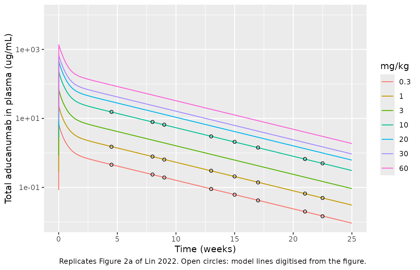
Figure 2a shows total plasma aducanumab after single 2-hour infusions of 0.3-60 mg/kg. The paper does not state the body weight used to convert mg/kg to an amount. The maintainers digitised the model lines of Figure 2a at times free of data symbols. In ug/mL the plotted concentration depends on body weight and not on the molar mass (which cancels between dose and output). A 70 kg patient reproduces the lines to within about 1%.

fig2a <- tibble::tribble(
  ~mgkg, ~week, ~Cc_fig,
  0.3, 4.5, 0.4549, 0.3, 8, 0.2364, 0.3, 9, 0.1936, 0.3, 13, 0.0902,
  0.3, 15, 0.0616, 0.3, 17, 0.0420, 0.3, 21, 0.0200, 0.3, 22.5, 0.0146,
  1, 4.5, 1.5099, 1, 8, 0.7848, 1, 9, 0.6425, 1, 13, 0.3049,
  1, 15, 0.2082, 1, 17, 0.1396, 1, 21, 0.0662, 1, 22.5, 0.0495,
  10, 4.5, 15.4694, 10, 8, 7.8953, 10, 9, 6.5830, 10, 13, 3.0126,
  10, 15, 2.0944, 10, 17, 1.4298, 10, 21, 0.6663, 10, 22.5, 0.4982
)

wt <- 70
sad_doses <- c(0.3, 1, 3, 10, 20, 30, 60)
sad_times <- sort(unique(c(0, 10^seq(-3, log10(25 * 7), length.out = 150), fig2a$week * 7)))
sad <- bind_rows(lapply(sad_doses, function(d) {
  ev <- rxode2::et(amt = d * wt, dur = 2 / 24, cmt = "central") |>
    rxode2::et(sad_times)
  solve(ui, ev) |> mutate(mgkg = d)
}))

# The time-0 row (no drug yet) cannot be drawn on a log axis.
ggplot(sad[sad$time != 0, ], aes(time / 7, Cc, colour = factor(mgkg))) +
  geom_line() +
  geom_point(data = fig2a, aes(week, Cc_fig), inherit.aes = FALSE, shape = 1) +
  scale_y_log10() +
  coord_cartesian(ylim = c(1e-2, 1e4)) +
  labs(
    x = "Time (weeks)", y = "Total aducanumab in plasma (ug/mL)", colour = "mg/kg",
    caption = "Replicates Figure 2a of Lin 2022. Open circles: model lines digitised from the figure."
  )

cmp2a <- fig2a |>
  left_join(sad |> mutate(week = round(time / 7, 6)) |> select(mgkg, week, Cc), by = c("mgkg", "week")) |>
  mutate(ratio = Cc_fig / Cc)
stopifnot(nrow(cmp2a) == nrow(fig2a), !anyNA(cmp2a$Cc))
summary(cmp2a$ratio)
#>    Min. 1st Qu.  Median    Mean 3rd Qu.    Max. 
#>  0.9829  0.9922  1.0013  0.9997  1.0073  1.0121
stopifnot(abs(median(cmp2a$ratio) - 1) < 0.02, all(abs(cmp2a$ratio - 1) < 0.05))

Non-compartmental analysis of the SAD simulation

The paper reports no NCA. The check below confirms two properties of the PK layer. First, exposure is nearly dose-proportional across the 200-fold SAD range (Figure 2a’s lines are parallel). The small departure is target-mediated: binding to plaque and ADCP in brain ISF consume a fixed amount of drug, which is a slightly larger fraction of a small dose. AUC per mg therefore rises monotonically with dose, by about 1.4% from 0.3 to 60 mg/kg. Second, the drug is lost almost entirely through first-order plasma elimination, so AUC0-inf is 96-98% of Dose / (kclearmAb * Vplasma).

# 750 days is about 29 terminal half-lives; a longer grid decays into solver
# noise and gives PKNCA non-positive concentrations to log.
nca_times <- sort(unique(c(0, 10^seq(-3, log10(750), length.out = 300))))
sad_nca <- bind_rows(lapply(sad_doses, function(d) {
  ev <- rxode2::et(amt = d * wt, dur = 2 / 24, cmt = "central") |>
    rxode2::et(nca_times)
  solve(ui, ev) |> mutate(treatment = paste(d, "mg/kg"), id = 1L)
})) |>
  filter(!is.na(Cc)) |>
  select(id, treatment, time, Cc)
stopifnot(all(sad_nca$Cc >= 0))

dose_df <- tibble(
  id = 1L, treatment = paste(sad_doses, "mg/kg"),
  time = 0, amt = sad_doses * wt, dur = 2 / 24
)
conc_obj <- PKNCA::PKNCAconc(sad_nca, Cc ~ time | treatment + id)
dose_obj <- PKNCA::PKNCAdose(dose_df, amt ~ time | treatment + id, duration = "dur")
intervals <- data.frame(
  start = 0, end = Inf, cmax = TRUE, tmax = TRUE,
  aucinf.obs = TRUE, half.life = TRUE
)
nca_res <- PKNCA::pk.nca(PKNCA::PKNCAdata(conc_obj, dose_obj, intervals = intervals))

nca_tab <- as.data.frame(nca_res) |>
  filter(PPTESTCD %in% c("cmax", "tmax", "aucinf.obs", "half.life")) |>
  select(treatment, PPTESTCD, PPORRES) |>
  tidyr::pivot_wider(names_from = PPTESTCD, values_from = PPORRES) |>
  mutate(
    dose_mg = as.numeric(sub(" mg/kg", "", treatment)) * wt,
    auc_per_mg = aucinf.obs / dose_mg,
    fraction_plasma_elim = aucinf.obs * 1.4586e-6 * 86400 * 3 / dose_mg
  ) |>
  arrange(dose_mg)
nca_tab |>
  dplyr::rename(
    "Dose" = treatment, "Cmax (ug/mL)" = cmax, "Tmax (day)" = tmax,
    "AUC0-inf (ug*day/mL)" = aucinf.obs, "t1/2 (day)" = half.life,
    "Dose (mg)" = dose_mg, "AUC0-inf / dose" = auc_per_mg,
    "AUC x kclearmAb x V / dose" = fraction_plasma_elim
  ) |>
  knitr::kable(digits = 3, caption = "PKNCA on the simulated SAD profiles (70 kg).")

PKNCA on the simulated SAD profiles (70 kg).

Dose	Cmax (ug/mL)	Tmax (day)	t1/2 (day)	AUC0-inf (ug*day/mL)	Dose (mg)	AUC0-inf / dose	AUC x kclearmAb x V / dose
0.3 mg/kg	6.860	0.084	25.383	53.603	21	2.553	0.965
1 mg/kg	22.866	0.084	25.384	178.730	70	2.553	0.965
3 mg/kg	68.598	0.084	25.386	536.641	210	2.555	0.966
10 mg/kg	228.659	0.084	25.393	1793.529	700	2.562	0.969
20 mg/kg	457.318	0.084	25.401	3598.151	1400	2.570	0.972
30 mg/kg	685.979	0.084	25.407	5410.641	2100	2.576	0.974
60 mg/kg	1371.964	0.084	25.411	10877.773	4200	2.590	0.979

stopifnot(
  nrow(nca_tab) == length(sad_doses),
  # near dose proportionality over 0.3-60 mg/kg ...
  diff(range(nca_tab$auc_per_mg)) / mean(nca_tab$auc_per_mg) < 0.02,
  # ... with the target-mediated sink shrinking as dose rises
  all(diff(nca_tab$auc_per_mg) > 0),
  # nearly all of the dose is eliminated from plasma at kclearmAb
  all(nca_tab$fraction_plasma_elim > 0.95 & nca_tab$fraction_plasma_elim <= 1)
)

Brain penetration (Figure S2)

The model was calibrated to a CSF-to-plasma aducanumab concentration ratio of about 0.5% at steady state (Results; Figure S2).

ev <- rxode2::et(amt = 10 * wt, dur = 2 / 24, cmt = "central", ii = 28, addl = 12) |>
  rxode2::et(seq(0, 364, by = 1))
csf <- solve(ui, ev) |> mutate(ratio_pct = 100 * Ccsf / Cc)
trough_ratio <- csf$ratio_pct[csf$time == 363]
trough_ratio
#> [1] 0.5017325
stopifnot(length(trough_ratio) == 1, abs(trough_ratio - 0.5) < 0.05)

Plasma A-beta (Figure 2b)

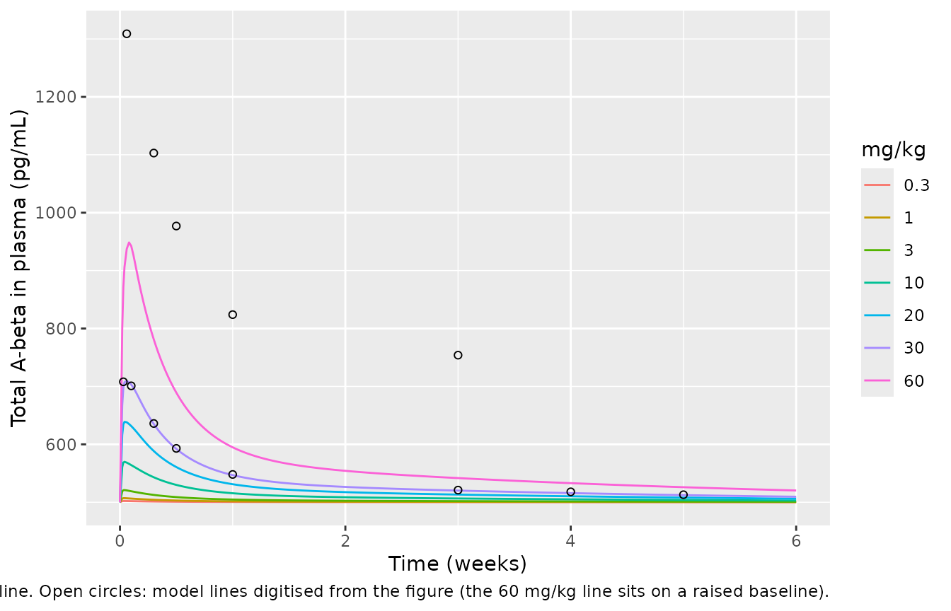
Total plasma A-beta (free plus drug-bound monomer and oligomer) rises after dosing because the drug-A-beta complex is cleared about 66-fold more slowly than free monomer. Figure 2b reports concentrations in pg/mL; the S3 plasma A-beta state (0.1155 nM) is drawn at 500 pg/mL, which corresponds to a molar mass of 4,330 g/mol (A-beta 1-40).

The 60 mg/kg group had a higher baseline (about 700 pg/mL), and the figure caption states that beta-secretase was raised for that group alone. The paper does not give the adjusted value. Total A-beta is linear in the amount of A-beta produced (drug binding to monomer is far from saturation), so the published 60 mg/kg curve should equal the nominal-baseline simulation times a constant. It does: the ratio stays within about 1.37-1.41 throughout.

fig2b <- tibble::tribble(
  ~mgkg, ~week, ~abeta_fig,
  30, 0.03, 708, 30, 0.1, 701, 30, 0.3, 636, 30, 0.5, 593,
  30, 1, 548, 30, 3, 521, 30, 4, 518, 30, 5, 513,
  # The 60 mg/kg line is not used at 0.03 weeks: it is still rising steeply
  # there, so a one-pixel error in time moves the digitised value by >5%.
  60, 0.06, 1309, 60, 0.3, 1103, 60, 0.5, 977,
  60, 1, 824, 60, 3, 754
)
b_times <- sort(unique(c(0, seq(0, 6 * 7, length.out = 300), fig2b$week * 7)))
sim2b <- bind_rows(lapply(sad_doses, function(d) {
  ev <- rxode2::et(amt = d * wt, dur = 2 / 24, cmt = "central") |>
    rxode2::et(b_times)
  solve(ui, ev) |> mutate(mgkg = d)
}))

ggplot(sim2b, aes(time / 7, abeta_plasma_total, colour = factor(mgkg))) +
  geom_line() +
  geom_point(data = fig2b, aes(week, abeta_fig), inherit.aes = FALSE, shape = 1) +
  labs(
    x = "Time (weeks)", y = "Total A-beta in plasma (pg/mL)", colour = "mg/kg",
    caption = paste(
      "Replicates Figure 2b of Lin 2022 at the nominal baseline. Open circles:",
      "model lines digitised from the figure (the 60 mg/kg line sits on a raised baseline)."
    )
  )

cmp2b <- fig2b |>
  left_join(sim2b |> mutate(week = round(time / 7, 6)) |> select(mgkg, week, abeta_plasma_total),
    by = c("mgkg", "week")
  ) |>
  mutate(ratio = abeta_fig / abeta_plasma_total)
stopifnot(nrow(cmp2b) == nrow(fig2b), !anyNA(cmp2b$ratio))
cmp2b |>
  dplyr::rename(
    "mg/kg" = mgkg, "Week" = week, "Figure 2b (pg/mL)" = abeta_fig,
    "Model (pg/mL)" = abeta_plasma_total, "Figure / model" = ratio
  ) |>
  knitr::kable(digits = 2)

mg/kg	Week	Figure 2b (pg/mL)	Model (pg/mL)	Figure / model
30	0.03	708	697.64	1.01
30	0.10	701	703.17	1.00
30	0.30	636	635.13	1.00
30	0.50	593	592.16	1.00
30	1.00	548	546.88	1.00
30	3.00	521	520.16	1.00
30	4.00	518	515.80	1.00
30	5.00	513	512.33	1.00
60	0.06	1309	937.30	1.40
60	0.30	1103	781.20	1.41
60	0.50	977	689.27	1.42
60	1.00	824	594.86	1.39
60	3.00	754	541.72	1.39

r30 <- cmp2b$ratio[cmp2b$mgkg == 30]
r60 <- cmp2b$ratio[cmp2b$mgkg == 60]
stopifnot(
  abs(sim2b$abeta_plasma_total[1] - 500) < 1,
  all(abs(r30 - 1) < 0.03),
  # constant scale factor on the raised 60 mg/kg baseline
  abs(median(r60) - 1.39) < 0.03, diff(range(r60)) < 0.06
)

Plaque reduction over one and two years (Figures 2c and 3a)

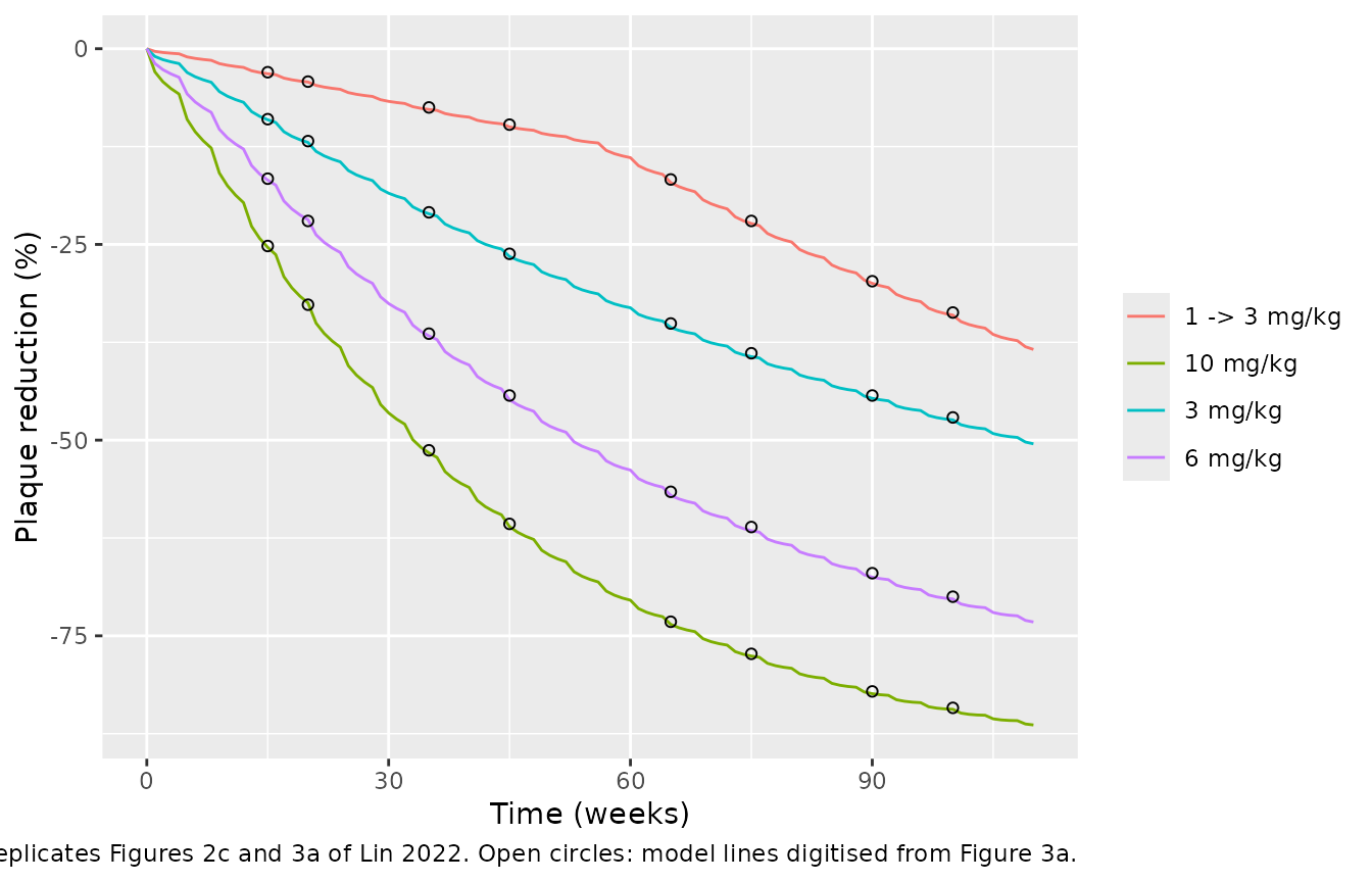
The paper compares the percent change of total brain plaque with the percent change of composite SUVR above a cutoff of 1.0. PRIME dosed every 4 weeks for one year (14 doses) and continued into a long-term extension (LTE) to week 110. In the LTE the 1 mg/kg group was switched to 3 mg/kg. The model curves of Figure 3a were digitised by the maintainers at times free of data symbols.

fig3a <- tibble::tribble(
  ~arm, ~week, ~pct_fig,
  "1 -> 3 mg/kg", 15, -3.0, "1 -> 3 mg/kg", 20, -4.2, "1 -> 3 mg/kg", 35, -7.5,
  "1 -> 3 mg/kg", 45, -9.7, "1 -> 3 mg/kg", 65, -16.7, "1 -> 3 mg/kg", 75, -22.0,
  "1 -> 3 mg/kg", 90, -29.7, "1 -> 3 mg/kg", 100, -33.7,
  "3 mg/kg", 15, -9.0, "3 mg/kg", 20, -11.8, "3 mg/kg", 35, -20.9, "3 mg/kg", 45, -26.2,
  "3 mg/kg", 65, -35.1, "3 mg/kg", 75, -38.9, "3 mg/kg", 90, -44.3, "3 mg/kg", 100, -47.1,
  "6 mg/kg", 15, -16.6, "6 mg/kg", 20, -22.0, "6 mg/kg", 35, -36.4, "6 mg/kg", 45, -44.3,
  "6 mg/kg", 65, -56.6, "6 mg/kg", 75, -61.1, "6 mg/kg", 90, -67.0, "6 mg/kg", 100, -70.0,
  "10 mg/kg", 15, -25.2, "10 mg/kg", 20, -32.7, "10 mg/kg", 35, -51.3, "10 mg/kg", 45, -60.7,
  "10 mg/kg", 65, -73.2, "10 mg/kg", 75, -77.3, "10 mg/kg", 90, -82.1, "10 mg/kg", 100, -84.2
)
arms <- list(
  "1 -> 3 mg/kg" = c(rep(1, 14), rep(3, 14)),
  "3 mg/kg" = rep(3, 28), "6 mg/kg" = rep(6, 28), "10 mg/kg" = rep(10, 28)
)
p_times <- sort(unique(c(seq(0, 110 * 7, by = 7), fig3a$week * 7)))
sim3a <- bind_rows(lapply(names(arms), function(a) {
  mg <- arms[[a]]
  ev <- rxode2::et(time = (seq_along(mg) - 1) * 28, amt = mg * wt, dur = 2 / 24, cmt = "central") |>
    rxode2::et(p_times)
  solve(ui, ev) |> mutate(arm = a)
}))

ggplot(sim3a, aes(time / 7, pct_plaque, colour = arm)) +
  geom_line() +
  geom_point(data = fig3a, aes(week, pct_fig), inherit.aes = FALSE, shape = 1) +
  labs(
    x = "Time (weeks)", y = "Plaque reduction (%)", colour = NULL,
    caption = "Replicates Figures 2c and 3a of Lin 2022. Open circles: model lines digitised from Figure 3a."
  )

cmp3a <- fig3a |>
  left_join(sim3a |> mutate(week = round(time / 7, 6)) |> select(arm, week, pct_plaque), by = c("arm", "week")) |>
  mutate(diff = pct_plaque - pct_fig)
stopifnot(nrow(cmp3a) == nrow(fig3a), !anyNA(cmp3a$diff))
c(mean = mean(cmp3a$diff), rms = sqrt(mean(cmp3a$diff^2)), max_abs = max(abs(cmp3a$diff)))
#>       mean        rms    max_abs 
#> -0.2756460  0.3225926  0.5365600
stopifnot(sqrt(mean(cmp3a$diff^2)) < 1, max(abs(cmp3a$diff)) < 2)

Dose titration (Figure 3b)

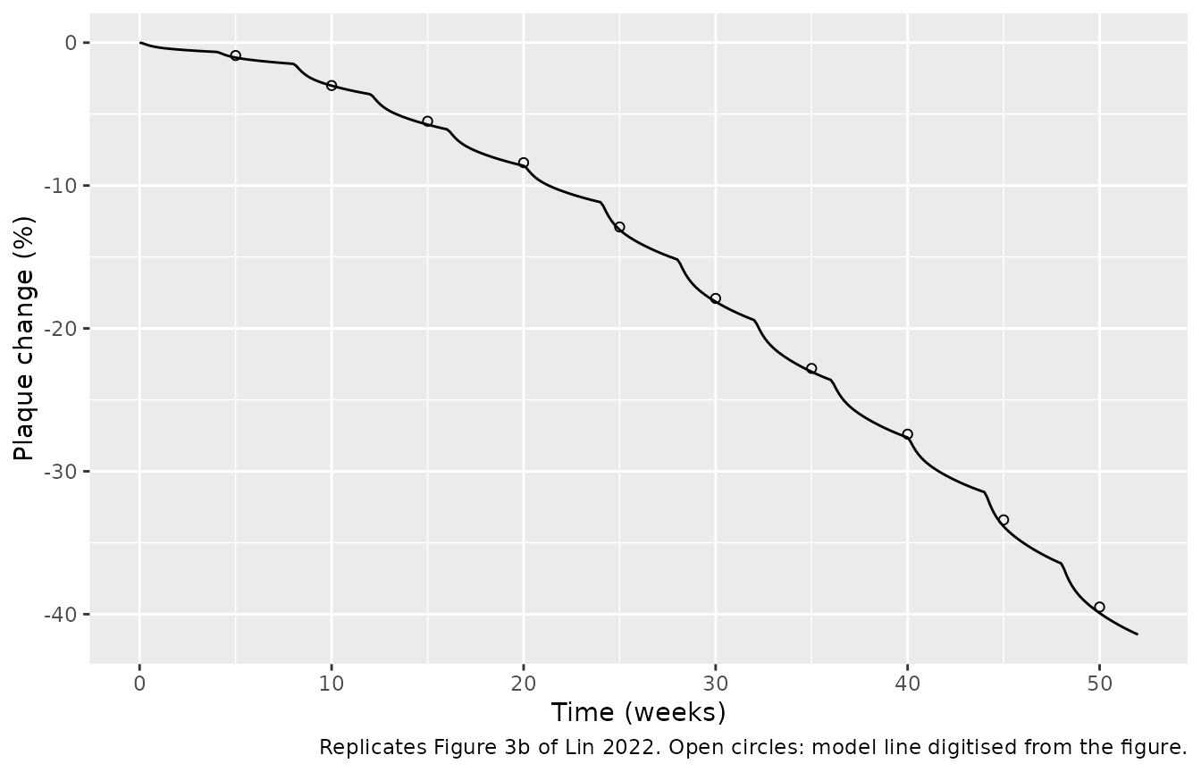
The titration cohort received 1 mg/kg for two doses, 3 mg/kg for four, 6 mg/kg for five and 10 mg/kg for two, all every 4 weeks. It was not used for calibration.

fig3b <- tibble::tribble(
  ~week, ~pct_fig,
  5, -0.9, 10, -3.0, 15, -5.5, 20, -8.4, 25, -12.9,
  30, -17.9, 35, -22.8, 40, -27.4, 45, -33.4, 50, -39.5
)
titr <- c(1, 1, 3, 3, 3, 3, 6, 6, 6, 6, 6, 10, 10)
ev <- rxode2::et(time = (seq_along(titr) - 1) * 28, amt = titr * wt, dur = 2 / 24, cmt = "central") |>
  rxode2::et(sort(unique(c(seq(0, 52 * 7, by = 1), fig3b$week * 7))))
sim3b <- solve(ui, ev)

ggplot(sim3b, aes(time / 7, pct_plaque)) +
  geom_line() +
  geom_point(data = fig3b, aes(week, pct_fig), shape = 1) +
  labs(
    x = "Time (weeks)", y = "Plaque change (%)",
    caption = "Replicates Figure 3b of Lin 2022. Open circles: model line digitised from the figure."
  )

cmp3b <- fig3b |>
  left_join(sim3b |> mutate(week = round(time / 7, 6)) |> select(week, pct_plaque), by = "week") |>
  mutate(diff = pct_plaque - pct_fig)
stopifnot(nrow(cmp3b) == nrow(fig3b), !anyNA(cmp3b$diff), max(abs(cmp3b$diff)) < 1.5)

Long-term treatment and recovery (Figure 4)

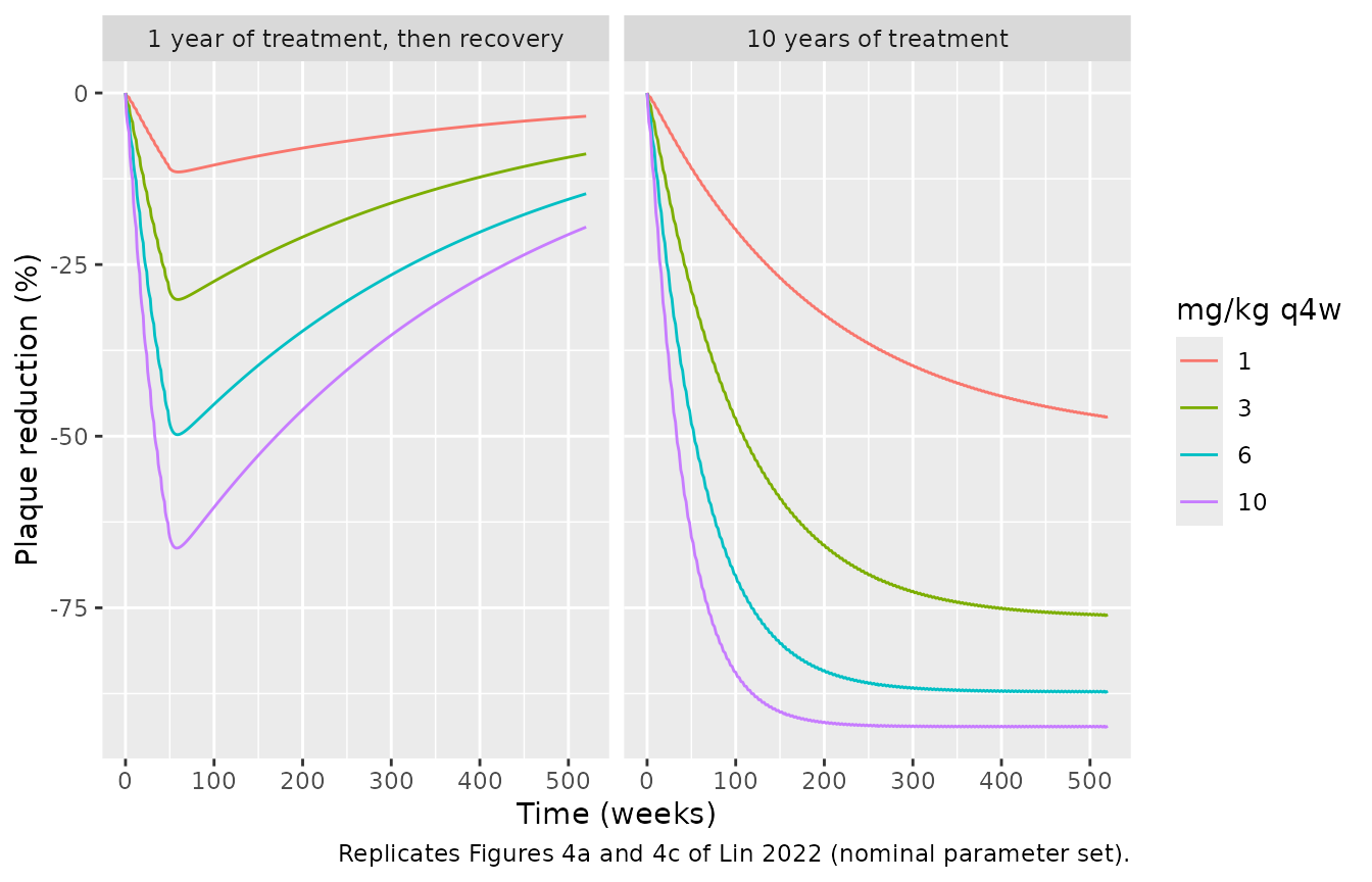
Figure 4a extends every-4-week dosing to 10 years, and Figure 4c stops after one year of treatment (13 doses) and follows plaque recovery to week 519. The endogenous plaque turnover is slow (about 25 years to steady state), so plaque recovers slowly.

fig4a <- tibble::tribble(
  ~mgkg, ~year, ~pct_fig,
  1, 1.5, -16.1, 1, 3, -27.4, 1, 5, -37.0, 1, 9.9, -46.8,
  3, 1.5, -40.2, 3, 3, -59.7, 3, 5, -70.5, 3, 9.9, -75.9,
  6, 1.5, -62.5, 6, 3, -80.7, 6, 5, -86.2, 6, 9.9, -87.2,
  10, 1.5, -78.2, 10, 3, -90.4, 10, 5, -92.2, 10, 9.9, -92.4
)
fig4c <- tibble::tribble(
  ~mgkg, ~week, ~pct_fig,
  1, 56, -11.3, 1, 100, -10.3, 1, 200, -7.9, 1, 300, -5.9, 1, 519, -3.5,
  3, 56, -29.7, 3, 100, -27.2, 3, 200, -20.7, 3, 300, -15.9, 3, 519, -8.7,
  6, 56, -49.1, 6, 100, -45.1, 6, 200, -34.3, 6, 300, -26.2, 6, 519, -14.7,
  10, 56, -65.7, 10, 100, -59.9, 10, 200, -45.8, 10, 300, -35.1, 10, 519, -19.5
)
yr <- 365.25
sim4a <- bind_rows(lapply(c(1, 3, 6, 10), function(d) {
  ev <- rxode2::et(amt = d * wt, dur = 2 / 24, cmt = "central", ii = 28, addl = 130) |>
    rxode2::et(sort(unique(c(seq(0, 10 * yr, by = 14), fig4a$year * yr))))
  solve(ui, ev) |> mutate(mgkg = d, regimen = "10 years of treatment")
}))
sim4c <- bind_rows(lapply(c(1, 3, 6, 10), function(d) {
  ev <- rxode2::et(amt = d * wt, dur = 2 / 24, cmt = "central", ii = 28, addl = 12) |>
    rxode2::et(sort(unique(c(seq(0, 520 * 7, by = 7), fig4c$week * 7))))
  solve(ui, ev) |> mutate(mgkg = d, regimen = "1 year of treatment, then recovery")
}))

bind_rows(sim4a, sim4c) |>
  ggplot(aes(time / 7, pct_plaque, colour = factor(mgkg))) +
  geom_line() +
  facet_wrap(~regimen) +
  labs(
    x = "Time (weeks)", y = "Plaque reduction (%)", colour = "mg/kg q4w",
    caption = "Replicates Figures 4a and 4c of Lin 2022 (nominal parameter set)."
  )

cmp4 <- bind_rows(
  fig4a |>
    left_join(sim4a |> mutate(year = round(time / yr, 6)) |> select(mgkg, year, pct_plaque), by = c("mgkg", "year")) |>
    mutate(panel = "4a"),
  fig4c |>
    left_join(sim4c |> mutate(week = round(time / 7, 6)) |> select(mgkg, week, pct_plaque), by = c("mgkg", "week")) |>
    mutate(panel = "4c")
) |>
  mutate(diff = pct_plaque - pct_fig)
stopifnot(nrow(cmp4) == nrow(fig4a) + nrow(fig4c), !anyNA(cmp4$diff))
cmp4 |>
  group_by(panel) |>
  summarise(rms = sqrt(mean(diff^2)), max_abs = max(abs(diff)))
#> # A tibble: 2 × 3
#>   panel   rms max_abs
#>   <chr> <dbl>   <dbl>
#> 1 4a    0.355   0.674
#> 2 4c    0.293   0.578
stopifnot(sqrt(mean(cmp4$diff^2)) < 1.5, max(abs(cmp4$diff)) < 3)

Soluble oligomer (Figure 5)

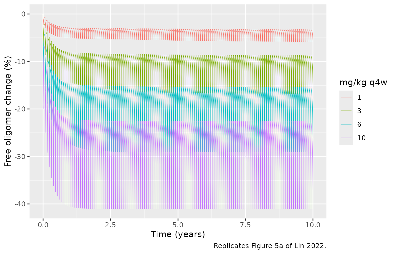
The model assumes that aducanumab clears soluble oligomer through ADCP with the same rate constants as plaque. Figure 5 shows the resulting band of free oligomer in brain ISF, which oscillates with each 4-weekly dose. The published 10 mg/kg band spans about -22% to -43% at steady state.

sim5 <- bind_rows(lapply(c(1, 3, 6, 10), function(d) {
  ev <- rxode2::et(amt = d * wt, dur = 2 / 24, cmt = "central", ii = 28, addl = 130) |>
    rxode2::et(seq(0, 10 * yr, by = 1))
  solve(ui, ev) |> mutate(mgkg = d)
}))
ggplot(sim5, aes(time / yr, pct_aolig_free, colour = factor(mgkg))) +
  geom_line(linewidth = 0.2) +
  labs(
    x = "Time (years)", y = "Free oligomer change (%)", colour = "mg/kg q4w",
    caption = "Replicates Figure 5a of Lin 2022."
  )

# The trough of free oligomer falls within hours of each infusion, so the band
# is measured on a fine grid over the last year rather than the daily grid
# used for the plot.
ev10 <- rxode2::et(amt = 10 * wt, dur = 2 / 24, cmt = "central", ii = 28, addl = 130) |>
  rxode2::et(seq(9 * yr, 10 * yr, by = 0.02))
band10 <- range(solve(ui, ev10)$pct_aolig_free)
band10
#> [1] -43.70380 -22.57304
stopifnot(abs(band10[1] - (-43)) < 1.5, abs(band10[2] - (-22)) < 1.5)

Regimens with the same total dose (Figure 6)

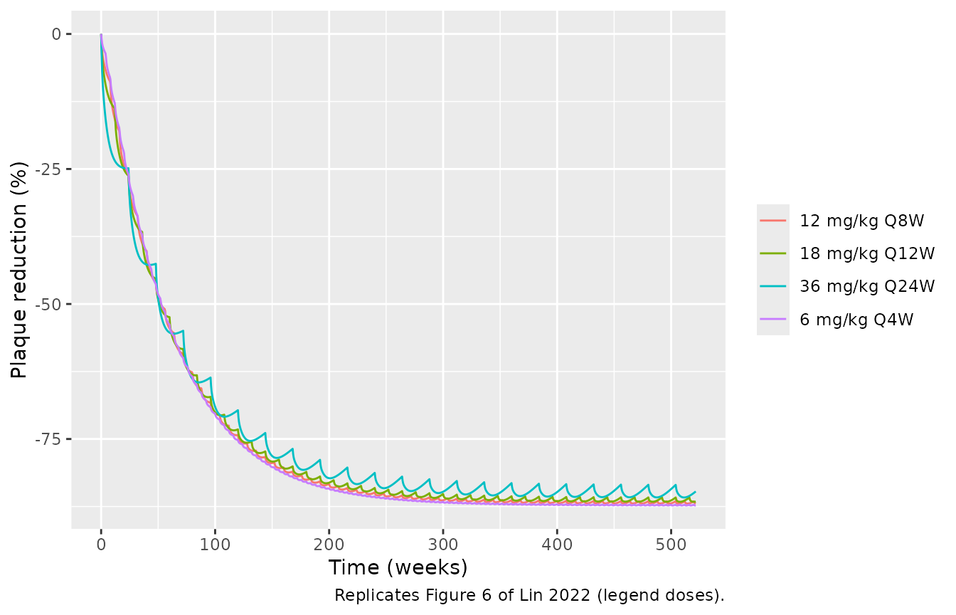
Figure 6 compares regimens with the same total dose and shows that they give nearly the same plaque reduction over 10 years. The figure legend lists 6 mg/kg every 4 weeks, 12 mg/kg every 8 weeks, 18 mg/kg every 12 weeks and 36 mg/kg every 24 weeks. The Results text and the caption instead list 10/20/30/60 mg/kg. The plotted plateau near -88% is the 6 mg/kg every-4-weeks plateau of Figure 4a; 10 mg/kg every 4 weeks plateaus at -92%. So the legend is correct, and the text and caption are in error.

regs <- tibble::tribble(
  ~label, ~mgkg, ~ii,
  "6 mg/kg Q4W", 6, 28, "12 mg/kg Q8W", 12, 56,
  "18 mg/kg Q12W", 18, 84, "36 mg/kg Q24W", 36, 168
)
sim6 <- bind_rows(lapply(seq_len(nrow(regs)), function(i) {
  n <- ceiling(10 * yr / regs$ii[i])
  ev <- rxode2::et(amt = regs$mgkg[i] * wt, dur = 2 / 24, cmt = "central", ii = regs$ii[i], addl = n - 1) |>
    rxode2::et(seq(0, 10 * yr, by = 3))
  solve(ui, ev) |> mutate(regimen = regs$label[i])
}))
ggplot(sim6, aes(time / 7, pct_plaque, colour = regimen)) +
  geom_line() +
  labs(
    x = "Time (weeks)", y = "Plaque reduction (%)", colour = NULL,
    caption = "Replicates Figure 6 of Lin 2022 (legend doses)."
  )

late6 <- sim6 |>
  filter(time > 8 * yr) |>
  group_by(regimen) |>
  summarise(min = min(pct_plaque), max = max(pct_plaque))
late6
#> # A tibble: 4 × 3
#>   regimen         min   max
#>   <chr>         <dbl> <dbl>
#> 1 12 mg/kg Q8W  -87.0 -86.5
#> 2 18 mg/kg Q12W -86.6 -85.8
#> 3 36 mg/kg Q24W -85.8 -83.4
#> 4 6 mg/kg Q4W   -87.3 -87.1
q4w_late <- late6$min[late6$regimen == "6 mg/kg Q4W"]
stopifnot(length(q4w_late) == 1, abs(q4w_late - (-88)) < 1.5, all(late6$min < -85))

Alternative parameter set (Figure 4b, Table S3)

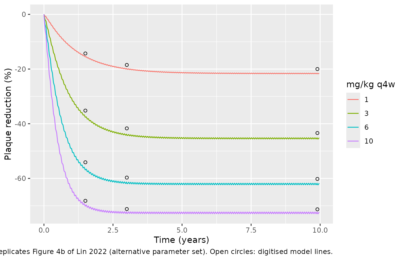
To show that the 1-year SUVR data cannot identify the endogenous plaque turnover, the authors recalibrated the model with plaque clearance fixed at five times its nominal value (Table S3). They then adjusted seven other parameters so that the 1-year data were still matched. This alternative set is a robustness exploration, not the final model: it fails to predict the week-110 SUVR data. It is not shipped as a separate model but can be applied with ini().

The alternative set has a different pretreatment steady state, and S3 gives only the nominal one. The simulation below therefore first runs the model untreated for 200 years. It then starts the dosing simulation from that state (passed as inits), and measures plaque change relative to the plaque at the first dose.

s2d <- 86400
alt <- suppressMessages(mod |>
  rxode2::ini(
    lkclearaplaq = log(5 * 4.4080e-09 * s2d),
    lkoffma2 = log(2.0e-02 / 1.5 * s2d),
    lkm2g = log(3 * 1.4e-05 * s2d),
    lkg2p = log(5 * 7.0e-08 * s2d),
    lk31abeta = log(4.1667e-05 / 1.5 * s2d),
    lk31aolig = log(4.1667e-05 / 1.5 * s2d),
    lk31bace = log(4.1667e-05 / 1.5 * s2d),
    lk31mab = log(4.1667e-05 / 1.5 * s2d),
    lk31mix = log(4.1667e-05 / 1.5 * s2d),
    lk43abeta = log(1.5509e-05 / 1.5 * s2d),
    lk43aolig = log(2.3264e-08 / 1.5 * s2d),
    lk43bace = log(1.5509e-05 / 1.5 * s2d),
    lk43mab = log(1.5509e-05 / 1.5 * s2d),
    lk43mix = log(2.3264e-08 / 1.5 * s2d),
    lksynthapp_plasma = log(1.2 * 1.44405e-03 * s2d),
    lksynthapp_bisf = log(3 * 2.5127e-04 * s2d)
  ))
runin <- solve(alt, rxode2::et(c(0, 200 * yr)))
alt_ss <- unlist(runin[2, ui$state])
fig4b <- tibble::tribble(
  ~mgkg, ~year, ~pct_fig,
  1, 1.5, -14.3, 1, 3, -18.5, 1, 9.9, -20.0,
  3, 1.5, -35.2, 3, 3, -41.7, 3, 9.9, -43.4,
  6, 1.5, -54.1, 6, 3, -59.7, 6, 9.9, -60.2,
  10, 1.5, -68.2, 10, 3, -71.2, 10, 9.9, -71.3
)
sim4b <- bind_rows(lapply(c(1, 3, 6, 10), function(d) {
  ev <- rxode2::et(amt = d * wt, dur = 2 / 24, cmt = "central", ii = 28, addl = 130) |>
    rxode2::et(sort(unique(c(seq(0, 10 * yr, by = 14), fig4b$year * yr))))
  solve(alt, ev, inits = alt_ss) |>
    mutate(
      mgkg = d, year = round(time / yr, 6),
      pct = 100 * (plaque_bisf / plaque_bisf[1] - 1)
    )
}))
alt_base <- sim4b$plaque_bisf[sim4b$mgkg == 1][1]
c(alt_baseline_plaque_nM = alt_base, nominal_baseline_plaque_nM = 1502.537143 / 0.261)
#>     alt_baseline_plaque_nM nominal_baseline_plaque_nM 
#>                   6015.912                   5756.847

ggplot(sim4b, aes(year, pct, colour = factor(mgkg))) +
  geom_line() +
  geom_point(data = fig4b, aes(year, pct_fig), inherit.aes = FALSE, shape = 1) +
  labs(
    x = "Time (years)", y = "Plaque reduction (%)", colour = "mg/kg q4w",
    caption = "Replicates Figure 4b of Lin 2022 (alternative parameter set). Open circles: digitised model lines."
  )

cmp4b <- fig4b |>
  left_join(sim4b |> select(mgkg, year, pct), by = c("mgkg", "year")) |>
  mutate(diff = pct - pct_fig)
stopifnot(nrow(cmp4b) == nrow(fig4b), !anyNA(cmp4b$diff))
c(mean = mean(cmp4b$diff), max_abs = max(abs(cmp4b$diff)))
#>      mean   max_abs 
#> -1.948578  2.788940
stopifnot(max(abs(cmp4b$diff)) < 4)

The alternative set reproduces Figure 4b to within a few percentage points. It is less exact than the nominal set because Table S3 reports the adjustments only as rounded fold changes (“1.5-fold decrease”, “3-fold increase”).

Assumptions and deviations

• Parameter conflicts. The deposited model code and Table S2 disagree on ksynthAPP_plasma, ksynthBACE_plasma, kG2M_bisf, koffma0 and koffma1/koffma2. Each was settled against a published model output (the S3 steady state, Figure 2b, or Figures 2c/3a and the text); see Parameter conflicts above. No value was tuned: every value used is printed in the code, in Table S2, or follows exactly from the published steady state.
• Body weight and molar masses (non-paper-derived). The paper gives doses in mg/kg and simulated in nmol but prints neither the body weight nor the molar masses. The maintainers inferred all three from the paper’s own figures: 70 kg from the Figure 2a lines (within about 1%); 150,000 g/mol for aducanumab from the Figure 3a plaque curves (root-mean-square error 0.3 percentage points, against 1.0 at the sequence-derived 145,912 g/mol that another model in this library uses); and 4,330 g/mol for A-beta from the 500 pg/mL baseline of Figure 2b. The model takes doses in mg; for a mg/kg regimen, multiply by the patient’s weight.
• APP input. The model code writes APP synthesis through an input APP_IN. The paper switches this input off only to simulate the SILK labelling experiment used in calibration (Figure S1). Every other simulation has it on, so it is encoded here as a constant synthesis rate. The SILK simulation is not reproduced.
• 60 mg/kg baseline. Figure 2b’s 60 mg/kg group was simulated with a raised beta-secretase level that the paper does not report. This article compares that curve after scaling by a constant factor (see Figure 2b above).
• Figure 6 doses. The Results text and the Figure 6 caption give 10, 20, 30 and 60 mg/kg; the legend and the plotted plateau correspond to 6, 12, 18 and 36 mg/kg. The legend doses are used.
• Equation typos in S4. The typeset equations (S4) differ from the model code in a few places. They show a negative sign on A-beta formation in brain ISF, drug-oligomer binding in brain ISF driven by CSF oligomer, and no oligomer-FcR binding term in the FcR equation. The model follows the reaction list of the deposited code, which is internally consistent and reproduces the published steady state and figures.
• Deterministic model. No between-subject variability or residual error is reported, and none is included.
• Errata. No correction notice for this article was found as of 2026-09-30.