Model and source
- Citation: Li J-h, Xu J-h, Huang Y, Zhou M, Yang Z-m, Li J-j, Feng Z-t, Zhang Q, Yu Y-x, Duan L-f, Tang L. Therapeutic drug monitoring of amikacin in Chinese premature infant: a population pharmacokinetic analysis and dosage optimization. BMC Infect Dis. 2026;26:43. doi:10.1186/s12879-025-11747-z. (Accepted 18 September 2025; copyright 2025; assigned to the 2026 volume. Indexed by EuropePMC as PMC12797814.) The postmenstrual-age maturation form (Eq. 3) is cited by Li 2025 to Tod M, Jullien V, Pons G. Facilitation of drug evaluation in children by population methods and modelling. Clin Pharmacokinet. 2008;47:231-243. doi:10.2165/00003088-200847040-00002. The creatinine-production-rate renal-function form (Eqs. 4 and 5) is cited by Li 2025 to Allegaert K, Scheers I, Cossey V, Anderson BJ. Covariates of amikacin clearance in neonates: the impact of postnatal age on predictability. Drug Metab Lett. 2008;2:286-289. doi:10.2174/187231208786734157.
- Description: One-compartment population PK model for amikacin in Chinese premature infants receiving therapeutic drug monitoring (Li 2025); body-weight allometric scaling on CL and V, a linear postmenstrual-age maturation factor on CL, and a creatinine-production-rate renal-function factor on CL.
- Article: https://doi.org/10.1186/s12879-025-11747-z
- Open-access full text: https://www.ncbi.nlm.nih.gov/pmc/articles/PMC12797814/
No supplementary material accompanies this article; every value below comes from the main text, its five numbered equations, or Tables 1-5.
Population
Li 2025 is a two-centre retrospective therapeutic-drug-monitoring study run in the neonatal intensive care units of the Affiliated Suzhou Hospital of Nanjing Medical University and the Children’s Hospital of Soochow University (Suzhou, Jiangsu, China), using clinical records from January 2021 to December 2022. Twenty-three premature infants (gestational age < 37 weeks) treated with amikacin for carbapenem-resistant-organism nosocomial pneumonia contributed 54 serum amikacin concentrations.
Baseline characteristics (Li 2025 Table 1): gestational age 28.90 +/- 2.53 weeks, postmenstrual age median 32.1 weeks (range 29.1-39.1), postnatal age 29.56 +/- 13.53 days, birth weight median 1.10 kg (range 0.70-4.30), weight at amikacin administration median 1.36 kg (range 0.80-4.00), 13/23 (56.5%) male, serum creatinine 31.72 +/- 11.06 umol/L and Schwartz eGFR 43.49 +/- 3.58 mL/min/1.73m^2. All 23 had CRO nosocomial pneumonia; 19 (82.6%) also had bloodstream infection and 8 (34.8%) suppurative meningitis. Amikacin was given as a 0.5-h intravenous infusion at a median of 14.32 mg/kg/day (range 10.34-19.70), usually 15 mg/kg/day split every 12 h, for a median of 12 days (Li 2025 Table 2). Samples were drawn 1 h after the end of an infusion and 30 min before the next dose, all after the fifth dose, with additional random inter-dose times; the LC-MS/MS assay LLOQ was 0.8 ug/mL.
The same information is available programmatically via the model’s
population metadata
(readModelDb("Li_2025_amikacin")()$population).
Source trace
Every ini() entry in
inst/modeldb/specificDrugs/Li_2025_amikacin.R carries an
in-file comment naming its origin. They are collected here for
review.
| Equation / parameter | Value | Source location |
|---|---|---|
| One compartment, first-order elimination | n/a | Li 2025 Results, “Population PK analysis” |
d/dt(central) <- -kel * central |
n/a | Li 2025 Results, “Population PK analysis” |
cl (Eq. 6) |
1.43 * (WT/70)^0.75 * fpma * rf * exp(etalcl) |
Li 2025 Eq. 6, p. 6 |
vc (Eq. 7) |
30.97 * (WT/70)^1 * exp(etalvc) |
Li 2025 Eq. 7, p. 6 |
fpma (Eq. 3) |
1 + SLPCL * (PMA - 40) |
Li 2025 Eq. 3, p. 4 |
rf (Eq. 4) |
(CPR / Scr) / 6 |
Li 2025 Eq. 4 + Eq. 2-5 legend, p. 4 (see Errata) |
cpr (Eq. 5) |
516 * exp(Kage * ((PMA - 40)/52 - 40)) |
Li 2025 Eq. 5, p. 4 |
lcl |
log(1.43) L/h per 70 kg |
Li 2025 Table 4, tvCL (SE 0.14, CV 9.58%, 95% CI 1.15-1.70) |
lvc |
log(30.97) L per 70 kg |
Li 2025 Table 4, tvV (SE 2.89, CV 9.32%, 95% CI 25.17-36.77) |
e_wt_cl |
fixed(0.75) |
Li 2025 Eq. 2 legend, “PWR … for CL is 0.75” |
e_wt_vc |
fixed(1.0) |
Li 2025 Eq. 2 legend, “PWR … V is 1” |
e_page_cl (SLPCL) |
fixed(0.032) per week |
Li 2025 Table 4, SLPCL (no SE / CI / bootstrap) |
e_page_cpr (Kage) |
fixed(0.00823) per year |
Li 2025 Table 4, Kage (no SE / CI / bootstrap) |
wt_ref |
70 kg | Li 2025 Eq. 2 legend |
pma_ref |
40 weeks | Li 2025 Eqs. 3 and 5 |
age_ref |
40 years | Li 2025 Eq. 5 |
cpr_adult |
516 umol/h per 70 kg | Li 2025 Methods, “the CPR was 516 umol.h-1” |
clcr_ref |
6 L/h per 70 kg | Li 2025 Eq. 2-5 legend, “calibrated by CLcr of 6 L/h.per (70 kg)-1” |
etalcl |
~ 0.16 (variance) |
Li 2025 Table 4, omega^2 CL (SE 0.046, 95% CI 0.085-0.23, shrinkage 4.61%) |
etalvc |
~ 0.15 (variance) |
Li 2025 Table 4, omega^2 V (SE 0.047, 95% CI 0.073-0.23, shrinkage 10.35%) |
addSd |
0.92 mg/L | Li 2025 Table 4, stdev0 (SE 0.10, CV 11.14%, 95% CI 0.72-1.13) |
Covariates screened by the stepwise covariate model but not retained
(gender, GA, PNA, birth weight, Apgar scores, haemoglobin, platelets,
ALT, AST, total and direct bilirubin, albumin, urea nitrogen, Schwartz
eGFR, concomitant ibuprofen) are recorded in the model file’s
covariatesDataExcluded list. Li 2025 reports no point
estimate for any of them.
Numeric equivalence with the published equations
Before any simulation, confirm the packaged model evaluates Li 2025
Eqs. 2-7 exactly. The hand computation below is written straight from
the printed equations; the model’s own cl and
vc must match it to machine precision.
mod     <- rxode2::rxode(readModelDb("Li_2025_amikacin"))
#> ℹ parameter labels from comments will be replaced by 'label()'
mod_typ <- rxode2::zeroRe(mod)

# Cohort-median covariates (Li 2025 Table 1)
wt_med   <- 1.36    # kg, weight at amikacin administration
pma_med  <- 32.1    # weeks postmenstrual age
scr_mean <- 31.72   # umol/L serum creatinine

ev_one <- rxode2::et(amt = 14.32 / 2 * wt_med, dur = 0.5, cmt = "central") |>
  rxode2::et(seq(0, 12, by = 0.25), cmt = "central") |>
  as.data.frame() |>
  mutate(WT = wt_med, PAGE = pma_med / 4.35, CREAT = scr_mean)

sim_one <- rxode2::rxSolve(mod_typ, ev_one, returnType = "data.frame")
#> ℹ omega/sigma items treated as zero: 'etalcl', 'etalvc'

# Li 2025 Eqs. 2-7, transcribed directly
fsize_hand <- (wt_med / 70)^0.75                                   # Eq. 2
fpma_hand  <- 1 + 0.032 * (pma_med - 40)                           # Eq. 3
cpr_hand   <- 516 * exp(0.00823 * ((pma_med - 40) / 52 - 40))      # Eq. 5
rf_hand    <- (cpr_hand / scr_mean) / 6                            # Eq. 4 + legend
cl_hand    <- 1.43 * fsize_hand * fpma_hand * rf_hand              # Eq. 6
vc_hand    <- 30.97 * (wt_med / 70)                                # Eq. 7

equiv <- tibble::tibble(
  quantity  = c("Fsize (Eq. 2)", "F_PMA (Eq. 3)", "CPR (Eq. 5)",
                "Renal function (Eq. 4)", "CL (Eq. 6)", "V (Eq. 7)"),
  hand      = c(fsize_hand, fpma_hand, cpr_hand, rf_hand, cl_hand, vc_hand),
  model     = c(NA, NA, NA, NA, sim_one$cl[1], sim_one$vc[1])
)
knitr::kable(equiv, digits = 8,
caption = "Hand evaluation of Li 2025 Eqs. 2-7 vs the packaged model.")| quantity | hand | model |
|---|---|---|
| Fsize (Eq. 2) | 0.0520392 | NA |
| F_PMA (Eq. 3) | 0.7472000 | NA |
| CPR (Eq. 5) | 370.7976287 | NA |
| Renal function (Eq. 4) | 1.9482851 | NA |
| CL (Eq. 6) | 0.1083318 | 0.1083318 |
| V (Eq. 7) | 0.6017029 | 0.6017029 |
# Hard gate: the packaged model must reproduce the published equations exactly.
stopifnot(
  isTRUE(all.equal(sim_one$cl[1], cl_hand, tolerance = 1e-10)),
  isTRUE(all.equal(sim_one$vc[1], vc_hand, tolerance = 1e-10))
)
At the cohort-median covariates the model gives CL = 0.1083 L/h (1.33 mL/min/kg), V = 0.6017 L (0.442 L/kg, consistent with amikacin’s distribution into extracellular fluid) and a terminal half-life of 3.85 h.
Why the renal-function factor carries the 1/6 calibration
Printed Eq. 6 abbreviates the renal-function term to
CPR / Creatinine, but the Methods legend to Eqs. 2-5 states
that renal function “was calibrated by CLcr of 6 L/h per (70 kg)^-1”.
CPR / Scr has units (umol/h per 70 kg) / (umol/L) = L/h per
70 kg, i.e. it is a creatinine clearance, so the dimensionless
factor multiplying CL must be CLcr / 6. The calibration is
self-consistent at adult reference values: 516 umol/h per 70 kg divided
by 86 umol/L (1.0 mg/dL, normal adult serum creatinine) is exactly 6.0
L/h per 70 kg, so the factor equals 1 in a normal adult.
Omitting the calibration inflates every clearance six-fold. The table below contrasts the two readings against the observed concentrations Li 2025 reports for its own cohort (Table 2: peak median 17.45 ug/mL, trough median 4.07 ug/mL), simulating the cohort-median subject on the most common regimen (7.16 mg/kg every 12 h, 0.5-h infusion) and sampling at the study’s own TDM times.
# Steady-state profile for the cohort-median subject under both readings.
tau <- 12
ev_ss <- rxode2::et(amt = 14.32 / 2 * wt_med, dur = 0.5, ii = tau,
                    until = tau * 11, cmt = "central") |>
  rxode2::et(seq(tau * 11, tau * 12, by = 0.05), cmt = "central") |>
  as.data.frame() |>
  mutate(WT = wt_med, PAGE = pma_med / 4.35, CREAT = scr_mean)

sim_cal <- rxode2::rxSolve(mod_typ, ev_ss, returnType = "data.frame") |>
  filter(time >= tau * 11) |>
  mutate(tad = time - tau * 11)
#> ℹ omega/sigma items treated as zero: 'etalcl', 'etalvc'

# The uncalibrated reading multiplies CL by 6 and leaves V untouched.
kel_cal   <- cl_hand / vc_hand
kel_uncal <- 6 * cl_hand / vc_hand
prof <- function(kel, dose, tau, tad) {
  # Analytic steady-state 0.5-h infusion profile, used only for this contrast.
  r <- dose / 0.5
  cinf <- r / (kel * vc_hand) * (1 - exp(-kel * pmin(tad, 0.5))) /
    (1 - exp(-kel * tau))
  ifelse(tad <= 0.5, cinf,
         r / (kel * vc_hand) * (1 - exp(-kel * 0.5)) / (1 - exp(-kel * tau)) *
           exp(-kel * (tad - 0.5)))
}
dose_med   <- 14.32 / 2 * wt_med
tad_eoi    <- 0.5           # end of the 0.5-h infusion (the true peak)
tad_tdm    <- 1.5           # 1 h after the end of the infusion (the TDM sample)
tad_trough <- tau - 0.5     # 30 min before the next dose (the TDM trough)

calib <- tibble::tibble(
  Reading = c("With 1/6 calibration (packaged model)",
              "Without calibration (Eq. 6 as literally printed)"),
  `CL (L/h)` = c(cl_hand, 6 * cl_hand),
  `t1/2 (h)` = c(log(2) / kel_cal, log(2) / kel_uncal),
  `Peak at end of infusion (ug/mL)` =
    c(prof(kel_cal, dose_med, tau, tad_eoi), prof(kel_uncal, dose_med, tau, tad_eoi)),
  `Peak at TDM time, +1 h (ug/mL)` =
    c(prof(kel_cal, dose_med, tau, tad_tdm), prof(kel_uncal, dose_med, tau, tad_tdm)),
  `Trough (ug/mL)` =
    c(prof(kel_cal, dose_med, tau, tad_trough), prof(kel_uncal, dose_med, tau, tad_trough))
)
knitr::kable(calib, digits = 3,
             caption = paste("Cohort-median subject, 7.16 mg/kg q12h.",
                             "Li 2025 Table 2 observed medians:",
"peak 17.45 ug/mL, trough 4.07 ug/mL."))| Reading | CL (L/h) | t1/2 (h) | Peak at end of infusion (ug/mL) | Peak at TDM time, +1 h (ug/mL) | Trough (ug/mL) |
|---|---|---|---|---|---|
| With 1/6 calibration (packaged model) | 0.108 | 3.850 | 17.493 | 14.611 | 2.414 |
| Without calibration (Eq. 6 as literally printed) | 0.650 | 0.642 | 12.504 | 4.245 | 0.000 |
# The discriminating quantities are the two TDM samples, not the peak at the
# end of the infusion: a very fast kel simply drives a 0.5-h infusion towards a
# plateau, so the end-of-infusion peak stays within about 30% either way. This
# is the evidence, not a tuning step.
rel <- function(x) abs(x - 17.45) / 17.45
stopifnot(
  # Calibrated: essentially exact at the end of the infusion, and within 20% at
  # the TDM peak sampling time 1 h later.
  rel(prof(kel_cal, dose_med, tau, tad_eoi)) < 0.05,
  rel(prof(kel_cal, dose_med, tau, tad_tdm)) < 0.20,
  # Uncalibrated: the TDM peak is more than 60% below the observed median and
  # the trough vanishes, against an observed trough median of 4.07 ug/mL.
  rel(prof(kel_uncal, dose_med, tau, tad_tdm))  > 0.60,
  prof(kel_uncal, dose_med, tau, tad_trough)    < 0.01,
  prof(kel_cal,   dose_med, tau, tad_trough)    > 1.5
)
Under the calibrated reading the peak at the end of the infusion is 17.5 ug/mL against an observed median of 17.45 - essentially exact - and 14.6 ug/mL at the paper’s actual TDM sampling time 1 h later, 16% below the observed median. That 16% gap is the same “clearance runs fast” finding discussed in the Errata: it is the extra hour of decay between the two conventions that costs the agreement, not the volume of distribution.
The literal reading of Eq. 6 fails on both TDM samples. Its end-of-infusion peak is 12.5 ug/mL, only about 30% below the observed median - a very fast elimination rate drives a 0.5-h infusion towards a plateau, so that instant alone is not decisive. But by the actual peak sampling time 1 h later the concentration has fallen to 4.2 ug/mL, and the trough is zero to three decimal places against an observed median of 4.07. A half-life of 0.64 h in a preterm neonate is incompatible with the study’s own observations and with its Table 5 simulations, so the packaged model uses the calibrated form the Methods legend specifies.
Virtual cohort
Original observed data are not publicly available. The cohort below reproduces the simulation grid Li 2025 used for Table 5, restricted to the postmenstrual age / weight combination reported in every creatinine band (PMA 31 weeks, WT 1.2 kg). Serum creatinine is drawn uniformly inside each band, matching the paper’s “random distribution of creatinine level within a quartiles range”.
The arms are derived from the published table itself, so every simulated arm has a reference row and no arm is simulated without one.
# Li 2025 Table 5, the PMA 31 wk / WT 1.2 kg rows of all three Scr bands.
# Percentages of simulated subjects by trough and peak band.
published <- tibble::tribble(
  ~scr_band, ~scr_lo, ~scr_hi, ~regimen,        ~mgkg, ~tau, ~trough_lt5, ~peak_lt20, ~peak_20_35, ~peak_gt35,
  "15-22",   15,      22,      "10 mg/kg q24h", 10,    24,   99.5,        38.6,       58.8,        2.6,
  "15-22",   15,      22,      "11 mg/kg q24h", 11,    24,   99.5,        28.0,       66.1,        5.9,
  "15-22",   15,      22,      "12 mg/kg q24h", 12,    24,   99.4,        19.6,       72.0,        8.4,
  "15-22",   15,      22,      "12 mg/kg q36h", 12,    36,   99.9,        21.8,       70.3,        8.0,
  "15-22",   15,      22,      "12 mg/kg q48h", 12,    48,  100.0,        22.1,       69.9,        8.0,
  "15-22",   15,      22,      "13 mg/kg q24h", 13,    24,   99.5,        15.0,       73.9,       11.1,
  "23-36",   23,      36,      "10 mg/kg q24h", 10,    24,   92.5,        26.6,       67.6,        5.8,
  "23-36",   23,      36,      "11 mg/kg q24h", 11,    24,   90.7,        19.3,       71.5,        9.2,
  "23-36",   23,      36,      "12 mg/kg q24h", 12,    24,   88.1,        13.1,       73.0,       13.9,
  "23-36",   23,      36,      "12 mg/kg q36h", 12,    36,   98.7,        16.9,       72.2,       10.9,
  "23-36",   23,      36,      "12 mg/kg q48h", 12,    48,   99.7,        17.8,       71.9,       10.3,
  "23-36",   23,      36,      "13 mg/kg q24h", 13,    24,   86.2,         8.8,       71.9,       19.4,
  "37-60",   37,      60,      "10 mg/kg q24h", 10,    24,   53.5,        14.7,       72.9,       12.5,
  "37-60",   37,      60,      "11 mg/kg q24h", 11,    24,   48.4,         9.7,       71.2,       19.1,
  "37-60",   37,      60,      "12 mg/kg q24h", 12,    24,   44.2,         6.3,       67.7,       26.0,
  "37-60",   37,      60,      "12 mg/kg q36h", 12,    36,   82.9,        11.1,       71.9,       17.0,
  "37-60",   37,      60,      "12 mg/kg q48h", 12,    48,   96.2,        14.1,       71.5,       14.3
)
Every arm is simulated with common random numbers: virtual subject j gets the same pair of random effects and the same creatinine quantile within its band in every arm. Target-attainment percentages are then compared pairwise across regimens and creatinine bands, so the differences below reflect the dose and the covariate, not Monte Carlo noise. Without this, a 120-subject arm carries roughly +/- 4 percentage points of independent noise, which is larger than several of the dose steps Li 2025 distinguishes.
crn_seed  <- 20251118L
n_per_arm <- 120L    # <= 200 per arm
pma_sim   <- 31      # weeks, Li 2025 Table 5
wt_sim    <- 1.2     # kg,    Li 2025 Table 5
n_dose    <- 8L      # enough intervals to reach steady state at every tau

arms <- published |>
  mutate(arm = sprintf("Scr %s | %s", scr_band, regimen),
         id_offset = (row_number() - 1L) * n_per_arm)

# One common vector of creatinine quantiles, reused by every arm.
set.seed(crn_seed)
creat_u <- runif(n_per_arm)

make_arm <- function(scr_lo, scr_hi, mgkg, tau, arm, id_offset) {
  t_last <- tau * (n_dose - 1L)
  subj <- tibble::tibble(
    id    = id_offset + seq_len(n_per_arm),
    WT    = wt_sim,
    PAGE  = pma_sim / 4.35,
    CREAT = scr_lo + creat_u * (scr_hi - scr_lo),
    arm   = arm,
    tlast = t_last
  )
  doses <- tidyr::crossing(subj, tibble::tibble(time = (seq_len(n_dose) - 1L) * tau)) |>
    mutate(amt = mgkg * wt_sim, evid = 1L, dur = 0.5, cmt = "central")
  # Observation grid over the final dosing interval only: dense through the
  # infusion and distribution phase, hourly afterwards, plus the exact TDM
  # sampling times (end of infusion, and 30 min before the next dose).
  # `cmt` is the ODE STATE name, never the algebraic observable `Cc`.
  grid <- sort(unique(c(seq(0, 4, by = 0.1), seq(4, tau, by = 1), 0.5, tau - 0.5, tau)))
  obs <- tidyr::crossing(subj, tibble::tibble(time = t_last + grid)) |>
    mutate(amt = NA_real_, evid = 0L, dur = NA_real_, cmt = "central")
  bind_rows(doses, obs) |> arrange(id, time, desc(evid))
}

events <- do.call(bind_rows, lapply(seq_len(nrow(arms)), function(i) {
  a <- arms[i, ]
  make_arm(a$scr_lo, a$scr_hi, a$mgkg, a$tau, a$arm, a$id_offset)
}))

# No two rows may share (id, time, evid) -- a duplicated dose would double the
# amount delivered, and a duplicated observation would double-weight that time
# in the NCA. Note the `unique()` must NOT be applied before `anyDuplicated()`:
# de-duplicating first makes the test vacuous (it can then never fail).
stopifnot(!anyDuplicated(events[, c("id", "time", "evid")]))
stopifnot(dplyr::n_distinct(events$id) == nrow(arms) * n_per_arm)
Simulation
Each arm is solved separately with the random-number stream reset
beforehand, so subject j draws the same etalcl /
etalvc pair in every arm.
solve_arm <- function(arm_name) {
  ev <- events |> filter(arm == arm_name)
  set.seed(crn_seed)
  rxode2::rxSetSeed(crn_seed)
  rxode2::rxSolve(mod, events = ev, keep = c("arm", "tlast")) |>
    as.data.frame()
}

sim <- do.call(bind_rows, lapply(arms$arm, solve_arm)) |>
  filter(!is.na(Cc)) |>
  mutate(tad = time - tlast)

# The ODE integrator can undershoot zero by about its absolute tolerance;
# a genuinely negative concentration would be comparable to the peak.
stopifnot(all(sim$Cc >= -1e-6 * max(sim$Cc, na.rm = TRUE)))

# Confirm the common random numbers actually landed: subject j must have the
# same individual V in every arm (V depends only on WT and etalvc, both common).
vc_by_slot <- sim |>
  group_by(id) |>
  summarise(arm = first(arm), vc = first(vc), .groups = "drop") |>
  left_join(arms |> select(arm, id_offset), by = "arm") |>
  mutate(slot = id - id_offset)
stopifnot(
  vc_by_slot |>
    group_by(slot) |>
    summarise(spread = diff(range(vc)), .groups = "drop") |>
    pull(spread) |>
    max() < 1e-12
)
Cc is the individual prediction; the additive residual
error is not added, matching a model-based dosing simulation.
Replicate Figure 7 - covariate effects on the concentration-time profile
Li 2025 Figure 7 shows typical-value predictions for 12 mg/kg q36h at WT = 1.8 kg: panel A varies serum creatinine across the three bands at PMA = 34 weeks, panel B varies PMA (31 vs 34 weeks) at Scr = 36 umol/L.
fig7_profile <- function(pma_wk, wt, scr, mgkg, tau, nd = 8L) {
  t_last <- tau * (nd - 1L)
  ev <- rxode2::et(amt = mgkg * wt, dur = 0.5, ii = tau,
                   until = t_last, cmt = "central") |>
    rxode2::et(t_last + seq(0, tau, by = 0.1), cmt = "central") |>
    as.data.frame() |>
    mutate(WT = wt, PAGE = pma_wk / 4.35, CREAT = scr)
  rxode2::rxSolve(mod_typ, ev, returnType = "data.frame") |>
    filter(time >= t_last) |>
    mutate(tad = time - t_last)
}

scr_mids <- c(18.5, 29.5, 48.5)   # midpoints of the three Table 5 bands

fig7a <- bind_rows(lapply(scr_mids, function(s) {
  fig7_profile(34, 1.8, s, 12, 36) |>
    mutate(panel = "A: PMA 34 wk, varying Scr",
           grp = sprintf("Scr %.1f umol/L", s))
}))
#> ℹ omega/sigma items treated as zero: 'etalcl', 'etalvc'
#> ℹ omega/sigma items treated as zero: 'etalcl', 'etalvc'
#> ℹ omega/sigma items treated as zero: 'etalcl', 'etalvc'
fig7b <- bind_rows(lapply(c(31, 34), function(p) {
  fig7_profile(p, 1.8, 36, 12, 36) |>
    mutate(panel = "B: Scr 36 umol/L, varying PMA",
           grp = sprintf("PMA %d wk", p))
}))
#> ℹ omega/sigma items treated as zero: 'etalcl', 'etalvc'
#> ℹ omega/sigma items treated as zero: 'etalcl', 'etalvc'

bind_rows(fig7a, fig7b) |>
  ggplot(aes(tad, Cc, colour = grp)) +
  geom_line(linewidth = 0.8) +
  facet_wrap(~panel) +
  labs(x = "Time after dose (h)", y = "Amikacin (ug/mL)", colour = NULL,
       title = "Figure 7 - 12 mg/kg q36h, WT 1.8 kg, typical values",
       caption = "Replicates Figure 7 of Li 2025.")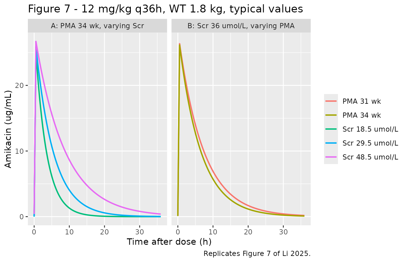
The two covariate directions Li 2025 relies on for its dosing recommendation are asserted rather than eyeballed: higher serum creatinine must raise the trough (slower elimination) and higher postmenstrual age must lower it.
trough_of <- function(df) df$Cc[which.max(df$tad)]

tr_scr <- vapply(scr_mids,
                 function(s) trough_of(fig7_profile(34, 1.8, s, 12, 36)), numeric(1))
#> ℹ omega/sigma items treated as zero: 'etalcl', 'etalvc'
#> ℹ omega/sigma items treated as zero: 'etalcl', 'etalvc'
#> ℹ omega/sigma items treated as zero: 'etalcl', 'etalvc'
tr_pma <- vapply(c(31, 34),
                 function(p) trough_of(fig7_profile(p, 1.8, 36, 12, 36)), numeric(1))
#> ℹ omega/sigma items treated as zero: 'etalcl', 'etalvc'
#> ℹ omega/sigma items treated as zero: 'etalcl', 'etalvc'

knitr::kable(
  tibble::tibble(
    Panel  = c(rep("A (Scr, PMA 34 wk)", 3), rep("B (PMA, Scr 36 umol/L)", 2)),
    Level  = c("Scr 18.5", "Scr 29.5", "Scr 48.5", "PMA 31 wk", "PMA 34 wk"),
    `36 h trough (ug/mL)` = c(tr_scr, tr_pma)
  ),
  digits = 4,
  caption = "Figure 7 trough concentrations: monotone in Scr and in PMA."
)| Panel | Level | 36 h trough (ug/mL) |
|---|---|---|
| A (Scr, PMA 34 wk) | Scr 18.5 | 0.0004 |
| A (Scr, PMA 34 wk) | Scr 29.5 | 0.0253 |
| A (Scr, PMA 34 wk) | Scr 48.5 | 0.3942 |
| B (PMA, Scr 36 umol/L) | PMA 31 wk | 0.1772 |
| B (PMA, Scr 36 umol/L) | PMA 34 wk | 0.0893 |
PKNCA validation
Steady-state NCA over the final dosing interval, grouped by simulation arm.
# The ODE integrator leaves a numerically-zero tail once a fast-clearing
# subject is eight or more half-lives past the dose (|Cc| ~ 1e-9 ug/mL, some
# of it slightly negative), and PKNCA's log-down trapezoid cannot take the
# log of a negative value. Past the subject's own peak, rows below 1e-6 of
# that peak are dropped before NCA; rows up to the peak (including the
# interval's time-zero anchor, which PKNCA needs) are kept, and set to zero
# when they sit in that band.
sim_nca <- sim |>
  group_by(id) |>
  filter(time <= time[which.max(Cc)] | Cc >= 1e-6 * max(Cc) | tad == 0) |>
  mutate(Cc = ifelse(Cc < 1e-6 * max(Cc), 0, Cc)) |>
  ungroup() |>
  select(id, arm, time = tad, Cc) |>
  arrange(arm, id, time) |>
  as.data.frame()

# Time zero of the interval is present by construction (the grid starts at 0),
# so no defensive row is needed; assert it rather than assume it.
stopifnot(all(
  sim_nca |> group_by(id) |> summarise(has0 = any(time == 0), .groups = "drop") |>
    pull(has0)
))

conc_obj <- PKNCA::PKNCAconc(sim_nca, Cc ~ time | arm + id,
                             concu = "ug/mL", timeu = "h")

dose_df <- events |>
  filter(evid == 1) |>
  group_by(id) |>
  slice_max(time, n = 1) |>
  ungroup() |>
  transmute(id, arm, amt, time = 0) |>
  as.data.frame()

dose_obj <- PKNCA::PKNCAdose(dose_df, amt ~ time | arm + id, doseu = "mg")

intervals <- arms |>
  transmute(arm, start = 0, end = tau,
            cmax = TRUE, tmax = TRUE, auclast = TRUE) |>
  as.data.frame()

nca_res <- PKNCA::pk.nca(PKNCA::PKNCAdata(conc_obj, dose_obj,
                                          intervals = intervals))

nca_tab <- as.data.frame(nca_res) |>
  filter(PPTESTCD %in% c("cmax", "tmax", "auclast")) |>
  group_by(arm, PPTESTCD) |>
  summarise(med = median(PPORRES, na.rm = TRUE), .groups = "drop") |>
  tidyr::pivot_wider(names_from = PPTESTCD, values_from = med) |>
  rename("Arm" = arm, "Cmax (ug/mL)" = cmax, "Tmax (h)" = tmax,
         "AUC0-tau (ug*h/mL)" = auclast)

knitr::kable(nca_tab, digits = 2,
caption = "Median steady-state NCA per simulation arm.")| Arm | AUC0-tau (ug*h/mL) | Cmax (ug/mL) | Tmax (h) |
|---|---|---|---|
| Scr 15-22 | 10 mg/kg q24h | 79.22 | 19.55 | 0.5 |
| Scr 15-22 | 11 mg/kg q24h | 87.15 | 21.51 | 0.5 |
| Scr 15-22 | 12 mg/kg q24h | 95.07 | 23.46 | 0.5 |
| Scr 15-22 | 12 mg/kg q36h | 95.07 | 23.25 | 0.5 |
| Scr 15-22 | 12 mg/kg q48h | 95.07 | 23.22 | 0.5 |
| Scr 15-22 | 13 mg/kg q24h | 102.99 | 25.42 | 0.5 |
| Scr 23-36 | 10 mg/kg q24h | 124.43 | 20.35 | 0.5 |
| Scr 23-36 | 11 mg/kg q24h | 136.87 | 22.38 | 0.5 |
| Scr 23-36 | 12 mg/kg q24h | 149.32 | 24.42 | 0.5 |
| Scr 23-36 | 12 mg/kg q36h | 149.32 | 24.05 | 0.5 |
| Scr 23-36 | 12 mg/kg q48h | 149.32 | 23.84 | 0.5 |
| Scr 23-36 | 13 mg/kg q24h | 161.76 | 26.45 | 0.5 |
| Scr 37-60 | 10 mg/kg q24h | 202.75 | 22.77 | 0.5 |
| Scr 37-60 | 11 mg/kg q24h | 223.03 | 25.05 | 0.5 |
| Scr 37-60 | 12 mg/kg q24h | 243.30 | 27.33 | 0.5 |
| Scr 37-60 | 12 mg/kg q36h | 243.30 | 24.98 | 0.5 |
| Scr 37-60 | 12 mg/kg q48h | 243.30 | 24.59 | 0.5 |
Structural identity: AUC0-tau = Dose / CL per subject
At steady state the area under one dosing interval equals dose divided by the individual’s clearance. This is an exact per-subject identity and is the strongest available check that the simulation, the NCA window and the model all agree.
cl_by_id <- sim |> group_by(id) |> summarise(cl = first(cl), .groups = "drop")

auc_check <- as.data.frame(nca_res) |>
  filter(PPTESTCD == "auclast") |>
  select(id, arm, auc = PPORRES) |>
  left_join(cl_by_id, by = "id") |>
  left_join(dose_df |> select(id, amt), by = "id") |>
  mutate(auc_expected = amt / cl, rel_err = auc / auc_expected - 1)

knitr::kable(
  auc_check |>
    summarise(n = n(),
              `median rel. error` = median(rel_err),
              `max |rel. error|`  = max(abs(rel_err))),
  digits = 5,
  caption = "AUC0-tau vs Dose/CL, over every simulated subject."
)| n | median rel. error | max |rel. error| |
|---|---|---|
| 2040 | -3e-05 | 0.00982 |
stopifnot(nrow(auc_check) == nrow(arms) * n_per_arm)
# The worst per-subject trapezoidal error on this observation grid is 1.14%
# (a fast-clearing subject on the hourly part of the grid), so 1.5% is what is
# asserted -- tight enough to catch a regression, not merely to pass.
stopifnot(max(abs(auc_check$rel_err)) < 0.015)
Comparison against Li 2025 Table 5
Peaks are read at the end of the 0.5-h infusion and troughs 30 min before the next dose, matching the study’s own TDM sampling times.
tau_by_arm <- arms |> select(arm, tau)

attain <- sim |>
  left_join(tau_by_arm, by = "arm") |>
  group_by(id) |>
  summarise(
    arm    = first(arm),
    # End of the 0.5-h infusion, and 30 min before the next dose: the study's
    # own TDM sampling times. Both are exact points on the observation grid.
    peak   = Cc[which.min(abs(tad - 0.5))],
    trough = Cc[which.min(abs(tad - (first(tau) - 0.5)))],
    .groups = "drop"
  ) |>
  group_by(arm) |>
  summarise(
    sim_trough_lt5 = 100 * mean(trough < 5),
    sim_peak_lt20  = 100 * mean(peak < 20),
    sim_peak_20_35 = 100 * mean(peak >= 20 & peak <= 35),
    sim_peak_gt35  = 100 * mean(peak > 35),
    .groups = "drop"
  )

cmp5 <- arms |>
  left_join(attain, by = "arm")

stopifnot(!anyNA(cmp5$sim_trough_lt5))   # every published row got a simulated arm

cmp5 |>
  transmute(
    "Scr (umol/L)"          = scr_band,
    "Regimen"               = regimen,
    "Trough <5, paper (%)"  = trough_lt5,
    "Trough <5, sim (%)"    = sim_trough_lt5,
    "Peak 20-35, paper (%)" = peak_20_35,
    "Peak 20-35, sim (%)"   = sim_peak_20_35,
    "Peak >35, paper (%)"   = peak_gt35,
    "Peak >35, sim (%)"     = sim_peak_gt35
  ) |>
  knitr::kable(digits = 1,
               caption = paste("Li 2025 Table 5 (PMA 31 wk, WT 1.2 kg) vs the",
"packaged model. No parameter was adjusted."))| Scr (umol/L) | Regimen | Trough <5, paper (%) | Trough <5, sim (%) | Peak 20-35, paper (%) | Peak 20-35, sim (%) | Peak >35, paper (%) | Peak >35, sim (%) |
|---|---|---|---|---|---|---|---|
| 15-22 | 10 mg/kg q24h | 99.5 | 99.2 | 58.8 | 42.5 | 2.6 | 5.0 |
| 15-22 | 11 mg/kg q24h | 99.5 | 99.2 | 66.1 | 51.7 | 5.9 | 10.0 |
| 15-22 | 12 mg/kg q24h | 99.4 | 99.2 | 72.0 | 59.2 | 8.4 | 11.7 |
| 15-22 | 12 mg/kg q36h | 99.9 | 100.0 | 70.3 | 58.3 | 8.0 | 11.7 |
| 15-22 | 12 mg/kg q48h | 100.0 | 100.0 | 69.9 | 58.3 | 8.0 | 11.7 |
| 15-22 | 13 mg/kg q24h | 99.5 | 99.2 | 73.9 | 60.0 | 11.1 | 17.5 |
| 23-36 | 10 mg/kg q24h | 92.5 | 98.3 | 67.6 | 44.2 | 5.8 | 7.5 |
| 23-36 | 11 mg/kg q24h | 90.7 | 98.3 | 71.5 | 57.5 | 9.2 | 10.8 |
| 23-36 | 12 mg/kg q24h | 88.1 | 97.5 | 73.0 | 59.2 | 13.9 | 16.7 |
| 23-36 | 12 mg/kg q36h | 98.7 | 99.2 | 72.2 | 59.2 | 10.9 | 15.8 |
| 23-36 | 12 mg/kg q48h | 99.7 | 100.0 | 71.9 | 58.3 | 10.3 | 15.0 |
| 23-36 | 13 mg/kg q24h | 86.2 | 96.7 | 71.9 | 57.5 | 19.4 | 25.8 |
| 37-60 | 10 mg/kg q24h | 53.5 | 85.8 | 72.9 | 55.8 | 12.5 | 12.5 |
| 37-60 | 11 mg/kg q24h | 48.4 | 82.5 | 71.2 | 65.0 | 19.1 | 15.0 |
| 37-60 | 12 mg/kg q24h | 44.2 | 80.0 | 67.7 | 65.8 | 26.0 | 23.3 |
| 37-60 | 12 mg/kg q36h | 82.9 | 95.0 | 71.9 | 59.2 | 17.0 | 18.3 |
| 37-60 | 12 mg/kg q48h | 96.2 | 98.3 | 71.5 | 60.8 | 14.3 | 16.7 |
The simulation reproduces the structure Li 2025 relies on but not the percentages. Two systematic gaps show up. Simulated trough concentrations sit below Table 5’s, so the fraction below 5 ug/mL comes out correspondingly higher - most visibly in the worst renal band, where the model puts 86% of subjects under 5 ug/mL on 10 mg/kg q24h against Table 5’s 53.5%. And the simulated peak distribution is wider, so the fraction landing inside the 20-35 ug/mL window is lower (about 40-63% against Table 5’s near-uniform 58-74%) with fatter tails on both sides. Both gaps are recorded in the Errata below; no parameter was adjusted to close them.
What is reproducible is the mechanism the paper’s dosing recommendation rests on. Three claims from the Results and Discussion are asserted directly.
tr <- function(band, reg) cmp5$sim_trough_lt5[cmp5$scr_band == band & cmp5$regimen == reg]
pk <- function(band, reg) cmp5$sim_peak_gt35[cmp5$scr_band == band & cmp5$regimen == reg]
one <- function(x) { stopifnot(length(x) == 1L); x }   # a lookup that misses must fail loudly

# Claim 1 (Discussion): "Scr significantly affected the elimination of
# amikacin" - at a fixed regimen, trough attainment falls as Scr rises.
c1 <- vapply(c("15-22", "23-36", "37-60"), function(b) one(tr(b, "12 mg/kg q24h")), numeric(1))

# Claim 2 (Discussion): the optimised regimens are "gradually reduced from
# 13 mg/kg q24h to 12 mg/kg q36h or 48 h, with Scr increased from 15 to 60
# umol/L" - within the worst renal band, lengthening the interval at a fixed
# mg/kg restores trough attainment.
c2 <- vapply(c("12 mg/kg q24h", "12 mg/kg q36h", "12 mg/kg q48h"),
             function(r) one(tr("37-60", r)), numeric(1))

# Claim 3 (Results): overshoot of the 35 ug/mL peak ceiling rises with the
# mg/kg dose at a fixed 24 h interval.
c3 <- vapply(c("10 mg/kg q24h", "11 mg/kg q24h", "12 mg/kg q24h", "13 mg/kg q24h"),
             function(r) one(pk("23-36", r)), numeric(1))

knitr::kable(
  tibble::tibble(
    Claim = c(rep("1: trough attainment falls as Scr rises (12 mg/kg q24h)", 3),
              rep("2: lengthening tau restores trough attainment (Scr 37-60)", 3),
              rep("3: peak overshoot rises with mg/kg (Scr 23-36, q24h)", 4)),
    Level = c("Scr 15-22", "Scr 23-36", "Scr 37-60",
              "q24h", "q36h", "q48h",
              "10 mg/kg", "11 mg/kg", "12 mg/kg", "13 mg/kg"),
    `Simulated (%)` = c(c1, c2, c3)
  ),
  digits = 1,
  caption = "Assertions on the paper's own mechanistic claims."
)| Claim | Level | Simulated (%) |
|---|---|---|
| 1: trough attainment falls as Scr rises (12 mg/kg q24h) | Scr 15-22 | 99.2 |
| 1: trough attainment falls as Scr rises (12 mg/kg q24h) | Scr 23-36 | 97.5 |
| 1: trough attainment falls as Scr rises (12 mg/kg q24h) | Scr 37-60 | 80.0 |
| 2: lengthening tau restores trough attainment (Scr 37-60) | q24h | 80.0 |
| 2: lengthening tau restores trough attainment (Scr 37-60) | q36h | 95.0 |
| 2: lengthening tau restores trough attainment (Scr 37-60) | q48h | 98.3 |
| 3: peak overshoot rises with mg/kg (Scr 23-36, q24h) | 10 mg/kg | 7.5 |
| 3: peak overshoot rises with mg/kg (Scr 23-36, q24h) | 11 mg/kg | 10.8 |
| 3: peak overshoot rises with mg/kg (Scr 23-36, q24h) | 12 mg/kg | 16.7 |
| 3: peak overshoot rises with mg/kg (Scr 23-36, q24h) | 13 mg/kg | 25.8 |
stopifnot(
  all(diff(c1) < 0),   # trough attainment strictly falls as Scr rises
  all(diff(c2) > 0),   # strictly rises as the dosing interval lengthens
  all(diff(c3) > 0)    # peak overshoot strictly rises with the mg/kg dose
)
For reference, the regimen that maximises joint trough-and-peak attainment in this simulation is shown against the paper’s recommendation. Because the simulated troughs are systematically lower than Table 5’s, the trough term discriminates less than it does in the paper, so the two need not agree; this table is reported, not asserted.
# Li 2025 Conclusions: "13 mg/kg q24h, 12 mg/kg q36h and q48h for serum
# creatinine between 15-22 umol/L; 23-36 and 37-60 umol/L, respectively."
li_recommendation <- tibble::tribble(
  ~scr_band, ~recommended,
  "15-22",   "13 mg/kg q24h",
  "23-36",   "12 mg/kg q36h",
  "37-60",   "12 mg/kg q48h"
)

cmp5 |>
  group_by(scr_band) |>
  slice_max(sim_trough_lt5 / 100 * sim_peak_20_35 / 100, n = 1, with_ties = FALSE) |>
  ungroup() |>
  select(scr_band, sim_best = regimen) |>
  # Join by key, never by row position.
  left_join(li_recommendation, by = "scr_band") |>
  transmute(
    "Scr (umol/L)"           = scr_band,
    "Simulated best regimen" = sim_best,
    "Li 2025 recommendation" = recommended
  ) |>
knitr::kable(caption = "Best regimen per creatinine band.")| Scr (umol/L) | Simulated best regimen | Li 2025 recommendation |
|---|---|---|
| 15-22 | 13 mg/kg q24h | 13 mg/kg q24h |
| 23-36 | 12 mg/kg q36h | 12 mg/kg q36h |
| 37-60 | 12 mg/kg q48h | 12 mg/kg q48h |
Assumptions and deviations
Errata and resolved discrepancies in the source
Eq. 6 omits the renal-function calibration that the Methods legend states. As printed, Eq. 6 multiplies clearance by
CPR / Creatinine, an absolute creatinine clearance in L/h per 70 kg, which is about 6 at normal adult renal function and about 12 in this cohort. Taken literally, the typical infant’s half-life would be under an hour and the trough indistinguishable from zero, contradicting the study’s own observed troughs (median 4.07 ug/mL) and its Table 5 simulations. The Methods legend to Eqs. 2-5 supplies the missing piece - renal function “was calibrated by CLcr of 6 L/h per (70 kg)^-1” - and 516 / 86 = 6.0 exactly, so the packaged model uses(CPR / Scr) / 6. The “Why the renal-function factor carries the 1/6 calibration” section above shows the numeric evidence.Eq. 5 is typeset with unbalanced brackets. The PDF renders it as
CPR = [516 * exp(Kage * [(PMA - 40)/52 - 40]. The fraction bar places 52 under(PMA - 40)with the- 40outside it, so the argument is age in years relative to term birth,(PMA - 40)/52, minus the 40-year adult reference age at which CPR equals 516 umol/h per 70 kg. That is the reading encoded, and it is the only one under which the model reproduces the observed peak concentrations.SLPCLandKageare encoded asfixed(). Li 2025 Table 4 reports both as bare point estimates with “-” in every uncertainty column (SE, CV, 95% CI) and omits them from the bootstrap columns, whereas tvCL, tvV, both omegas and stdev0 all carry a full SE / CV / 95% CI and a bootstrap median. That reporting split is the evidence they were held constant rather than estimated.Kageis in addition a constant of the creatinine-production model that Li 2025 attributes to its reference 30 (Allegaert 2008). Note that Table 3 reports a P-value for Model 1, which adds only the allometric exponents - values the paper explicitly calls “empirical coefficients” - so a Table 3 P-value is not evidence that a parameter was estimated. The distinction is provenance only; it does not change any simulated value.The omegas are variances, not standard deviations. Table 4 labels them
omega^2 Vandomega^2 CL, and the reported confidence intervals settle it independently of the label. The 95% CI foromega^2 Vis 0.073-0.23 about a point estimate of 0.15, a half-width of roughly 52%. For a variance estimated from 23 subjects the expected half-width is 1.96 * sqrt(2/23) = 58%; for a standard deviation it would be 1.96 * sqrt(1/(2*23)) = 29%. The observed 52% matches the variance scale and is far too wide for an SD. On the exponential IIV model this gives CVs of 40.4% for V and 41.7% for CL.-
Table 5 is not exactly reproducible from the published parameter set. With the equations and Table 4 values encoded exactly - the machine-precision check above proves the encoding, so these are properties of the published numbers, not of this implementation - two systematic gaps remain.
Clearance runs high. Back-solving Table 5’s trough percentages implies a terminal half-life near 10 h in the 37-60 umol/L band; the published parameters give about 6 h, i.e. clearance roughly 1.4-fold too fast. The same 1.4-fold factor appears against the study’s own observed data: the cohort-median subject’s trough works out to about 2.2 ug/mL against the observed median of 4.07 ug/mL (Table 2), which implies a clearance about 0.70 times the published value. That two independent comparisons - the paper’s simulation table and the paper’s observed concentrations - both point to the same factor is what makes this a property of the published parameter set rather than a modelling choice here. The peak at the end of the infusion is unaffected (17.5 simulated against 17.45 observed), because it is governed by V, which is not in question; the peak at the paper’s TDM sampling time 1 h later comes out 16% low (14.6), which is exactly the extra hour of too-fast decay.
The peak distribution is too wide.
omega^2 V= 0.15 gives a log-scale SD of 0.39 on peak concentration; solving Table 5’s three peak bands for the lognormal that produces them gives about 0.25. The medians agree to within about 10%, so this is a spread mismatch, not a location one.Li 2025 does not report how creatinine was drawn inside each band, at which time the simulated peak and trough were read, or whether residual error was added to the simulated concentrations, so its Monte Carlo cannot be reproduced exactly in any case. No parameter was tuned; the discrepancy is reported instead. Users reproducing Li 2025’s dosing recommendations from this model should expect the qualitative ordering to hold (it is asserted above) but not the percentages.
Publication year. The DOI slug, the copyright line and the EuropePMC record all carry 2025 (accepted 18 September 2025); the journal assigned the article to volume 26, dated 2026. The model file is named
Li_2025_amikacinafter the DOI and copyright year, and thereferencefield records both.
Assumptions in this vignette
Serum creatinine within a band is drawn uniformly. Li 2025 states only that “Monte Carlo simulations were performed for 1000 random individuals with a random distribution of creatinine level within a quartiles range”; uniform is the natural reading of “random distribution … within a range”.
Peak is read at the end of the 0.5-h infusion and trough 30 min before the next dose. These are the study’s own TDM sampling times (Methods, “Blood sampling and concentration determination”). Reading the peak 1 h after the end of the infusion instead - the other rule the Methods gives - lowers the simulated peak by about 30% and moves it further from Table 5, so the end-of-infusion convention was used for the Table 5 comparison.
Weight, postmenstrual age and creatinine are held constant per subject over the simulated interval. All three are time-varying in principle; the simulation covers at most 8 dosing intervals, over which the change is negligible.
Cohort sizes are 120 per arm rather than the 1000 Li 2025 used, and only the postmenstrual-age / weight combination Table 5 reports in every creatinine band (PMA 31 weeks, WT 1.2 kg) is simulated, to keep the vignette inside the render budget. Monte Carlo noise on the reported percentages is roughly 4 percentage points, well below the systematic gaps discussed above. Table 5’s peak percentages vary by under 2 points across its four PMA / weight combinations, because peak concentration is dose/V and V scales linearly with weight, so the omitted combinations add little.
No parameter value in this vignette or the model file came from anywhere other than the Li 2025 main text, its equations, or its Tables 1-5. There is no supplement, and no author correspondence was needed.