Tipifarnib (Perez-Ruixo 2006)
Source:vignettes/articles/PerezRuixo_2006_tipifarnib.Rmd
PerezRuixo_2006_tipifarnib.RmdModel and source
- Citation: Perez-Ruixo JJ, Piotrovskij V, Zhang S, Hayes S, De Porre P, Zannikos P. Population pharmacokinetics of tipifarnib in healthy subjects and adult cancer patients. Br J Clin Pharmacol. 2006;62(1):81-96. doi:10.1111/j.1365-2125.2006.02615.x
- Description: Three-compartment population PK model for oral and IV tipifarnib in healthy subjects and adult cancer patients (Perez-Ruixo 2006). Sequential zero-order release into the depot (duration D1) followed by first-order absorption (Ka) into the central compartment, with absorption lag time, linear elimination, two peripheral compartments, and bioavailability fixed at 26.7 percent. Covariate effects retained in the final model are total bilirubin on CL (power exponent -0.103 centred at 9 umol/L) and body weight on V2 (linear scaling, exponent fixed at 1, centred at 70 kg); healthy-vs-cancer cohort multipliers apply to CL, V2, Q4, V4, and Ka; a solution-vs-solid formulation indicator scales D1, Ka, and tlag. The mixture-model lag-time subpopulation (71.7 percent subpop 1 vs 28.3 percent subpop 2) is collapsed to the typical subpop-1 lag time for library simulation use; correlated IIVs with paper-reported correlation 1 (Q3-V3, CL-Q4, CL-V4) are encoded as derived etas via the published variance-expansion factors.
- Article: https://doi.org/10.1111/j.1365-2125.2006.02615.x
Population
The combined data set merges 15 clinical studies of orally and intravenously administered tipifarnib (Perez-Ruixo 2006 Tables 1 and 2): 1083 subjects (1035 adult cancer patients and 48 healthy subjects), 7339 plasma concentrations, dose range 25-1300 mg orally as solution / capsule / tablet (single or twice-daily) plus 1 h, 2 h, and 24 h IV infusions of 50-500 mg. Cancer indications include advanced breast cancer, small-cell lung cancer, advanced urothelial transitional-cell, superficial bladder cancer, advanced colorectal, advanced pancreatic cancers, and acute myeloid leukaemia (phase 2 and 3 studies plus six phase 1 cancer-patient cohorts). Healthy subjects came from two phase 1 cohorts (n = 12 in the index set, n = 36 in the test set after the model-development cutoff).
The pooled cohort had median age 60 years (range 18-89), median body weight 70.0 kg (range 34.0-145), 480/1083 (44.3 percent) female, and median total bilirubin 10.0 umol/L (range 2.0-116). Race was reported as 93.6 percent Caucasian, 1.8 percent African-American, and 4.5 percent Other (no separate Asian stratum), and was not retained as a structural covariate.
The same information is available programmatically via
readModelDb("PerezRuixo_2006_tipifarnib")$population.
Source trace
The per-parameter origin is recorded as an in-file comment next to
each ini() entry in
inst/modeldb/specificDrugs/PerezRuixo_2006_tipifarnib.R.
The table below collects them in one place for review.
| Equation / parameter | Value | Source location |
|---|---|---|
| Three-compartment disposition with sequential ZO -> FO absorption | n/a | Perez-Ruixo 2006 Figure 1 (compartmental schematic) and Results, Structural model selection (page 84) |
| CL (cancer, reference TBILI = 9 umol/L) | 21.9 L/h | Table 4, “Typical value Cancer subjects” column |
| V2 (cancer, per 70 kg) | 54.9 L | Table 4, “Typical value Cancer subjects” column |
| Q3 | 4.11 L/h | Table 4 (cancer = healthy) |
| V3 | 92.4 L | Table 4 (cancer = healthy) |
| Q4 (cancer) | 14.8 L/h | Table 4 |
| V4 (cancer) | 21.4 L | Table 4 |
| D1 (solid formulation) | 1.20 h | Table 4 |
| Ka (cancer, solid) | 0.71 1/h | Table 4 |
| F (absolute bioavailability) | 0.267 | Table 4 (Fabs = 26.7 percent) |
| tlag (solid, subpopulation 1) | 0.11 h | Table 4 |
| TBILI exponent on CL | -0.103 | Table 4 footnote a |
| WT exponent on V2 (fixed at 1) | 1 | Table 3 footnote 2 (power coefficient not different from 1) |
| Healthy:cancer CL ratio | 1.21 | Table 4 “Ratio healthy subjects : cancer subjects” |
| Healthy:cancer V2 ratio | 0.55 | Table 4 |
| Healthy:cancer Q4 ratio | 8.83 | Table 4 |
| Healthy:cancer V4 ratio | 2.66 | Table 4 |
| Healthy:cancer Ka ratio | 2.31 | Table 4 |
| Solution:solid D1 ratio | 0.348 | Table 4 footnote i |
| Solution:solid Ka ratio | 2.07 | Table 4 footnote j |
| Solution:solid tlag ratio | 0.183 | Table 4 footnote k |
| IIV CL | 24.9 percent CV | Table 4; corroborated in Discussion (“low between and within subject variabilities of 24.9 percent and 11.9 percent”) |
| IIV V2 | 20.3 percent CV | Table 4; corroborated in Discussion (“estimated to be 54.9 l 70 kg-1 (20.3 percent)”) |
| IIV Q3 | 74.0 percent CV | Table 4 |
| IIV D1 | 52.7 percent CV | Table 4 |
| IIV Ka | 86.1 percent CV | Table 4 |
| IIV F (logit-domain SD) | 0.74 | Table 4 footnote g (logit domain) |
| Variance expansion V3 / Q3 (corr = 1) | 1.21 | Table 4 footnote c |
| Variance expansion Q4 / CL (corr = 1) | 2.08 | Table 4 footnote d |
| Variance expansion V4 / CL (corr = 1) | 0.95 | Table 4 footnote e |
| Residual error (full PK profiles) | 24.5 percent CV | Table 4 footnote h |
Virtual cohort
Original observed data are not publicly available. The cohort below is a virtual population approximating the index data set (cancer patients on 300 mg twice-daily oral tablet), the dose level used in the most prominent published exposure-response analysis (Perez-Ruixo 2006 Discussion citing reference [9]).
set.seed(20250610)

n_per_arm <- 30L

make_cohort <- function(n, dis_healthy = 0L, form_solution = 0L, id_offset = 0L) {
  tibble::tibble(
    id           = id_offset + seq_len(n),
    WT           = rlnorm(n, meanlog = log(70), sdlog = 0.15),
    TBILI        = rlnorm(n, meanlog = log(9),  sdlog = 0.30),
    DIS_HEALTHY  = dis_healthy,
    FORM_SOLUTION = form_solution
  )
}

cohort <- dplyr::bind_rows(
  make_cohort(n_per_arm, dis_healthy = 0L, form_solution = 0L, id_offset =   0L) |>
    dplyr::mutate(treatment = "Cancer, solid"),
  make_cohort(n_per_arm, dis_healthy = 1L, form_solution = 0L, id_offset = 100L) |>
    dplyr::mutate(treatment = "Healthy, solid"),
  make_cohort(n_per_arm, dis_healthy = 0L, form_solution = 1L, id_offset = 200L) |>
    dplyr::mutate(treatment = "Cancer, solution")
)

# Build event tables per subject: 300 mg b.d. for 5 days, sampling out to 144 h.
# Use explicit dose times so the dose records survive as one row per dose event
# (needed for PKNCAdose downstream).
dose_times <- seq(0, 24 * 5, by = 12)
obs_times  <- seq(0, 24 * 6, by = 0.5)

make_events <- function(row) {
  ev <- rxode2::et(amt = 300, time = dose_times, cmt = "depot") |>
    rxode2::add.sampling(obs_times)
  ev <- as.data.frame(ev)
  ev$id <- row$id
  ev$WT <- row$WT
  ev$TBILI <- row$TBILI
  ev$DIS_HEALTHY <- row$DIS_HEALTHY
  ev$FORM_SOLUTION <- row$FORM_SOLUTION
  ev$treatment <- row$treatment
  ev
}

events <- do.call(
  rbind,
  lapply(split(cohort, cohort$id), make_events)
)
events <- events[order(events$id, events$time, events$evid), ]

stopifnot(!anyDuplicated(unique(events[, c("id", "time", "evid")])))
Simulation
mod <- readModelDb("PerezRuixo_2006_tipifarnib")
sim <- rxode2::rxSolve(mod, events = events, keep = c("treatment", "WT", "TBILI"))
#> ℹ parameter labels from comments will be replaced by 'label()'
sim <- as.data.frame(sim)
Replicate published figures
The paper reports simulations for 600 mg twice-daily; the chunk below reproduces the qualitative comparisons (steady-state profiles in healthy vs cancer subjects, and solid vs solution formulation) for the 300 mg twice-daily dose, which is the registered cancer dose used in the published exposure-response work.
# Replicates Figure 5A and 5B of Perez-Ruixo 2006: simulated steady-state
# plasma concentration vs time profiles by cohort (healthy vs cancer) and
# by formulation (solid vs solution) in cancer patients.
sim |>
  dplyr::filter(time >= 24 * 4 & time <= 24 * 5) |>  # final dosing interval
  dplyr::mutate(t_in_interval = time - 24 * 4) |>
  dplyr::group_by(treatment, t_in_interval) |>
  dplyr::summarise(
    Q10 = quantile(Cc, 0.10, na.rm = TRUE),
    Q50 = quantile(Cc, 0.50, na.rm = TRUE),
    Q90 = quantile(Cc, 0.90, na.rm = TRUE),
    .groups = "drop"
  ) |>
  ggplot(aes(t_in_interval, Q50, colour = treatment, fill = treatment)) +
  geom_ribbon(aes(ymin = Q10, ymax = Q90), alpha = 0.20, colour = NA) +
  geom_line(linewidth = 0.8) +
  scale_y_log10(name = "Plasma tipifarnib (ng/mL)") +
  scale_x_continuous(name = "Time since last dose (h)") +
  labs(
    title    = "Figure 5 - Simulated steady-state PK by cohort and formulation",
    subtitle = "300 mg b.d. multiple oral doses, last dosing interval",
    caption  = "Replicates Figures 5A (cohort) and 5B (formulation) of Perez-Ruixo 2006."
  ) +
  theme_minimal()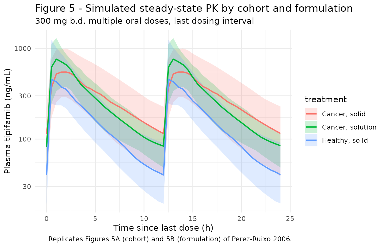
PKNCA validation
# Build PKNCA inputs over the final dosing interval (steady state, AUC0-tau).
tau <- 12

start_ss <- 24 * 4
end_ss   <- start_ss + tau

sim_nca <- sim |>
  dplyr::filter(!is.na(Cc)) |>
  dplyr::select(id, time, Cc, treatment)

# Defensively guarantee a time = 0 row per (id, treatment) so PKNCA's AUC
# integration anchors at the dose; for extravascular models pre-dose Cc = 0
# is the correct value.
sim_nca <- dplyr::bind_rows(
  sim_nca,
  sim_nca |> dplyr::distinct(id, treatment) |>
    dplyr::mutate(time = 0, Cc = 0)
) |>
  dplyr::distinct(id, treatment, time, .keep_all = TRUE) |>
  dplyr::arrange(id, treatment, time)

conc_obj <- PKNCA::PKNCAconc(
  sim_nca,
  Cc ~ time | treatment + id,
  concu = "ng/mL",
  timeu = "h"
)

dose_df <- events |>
  dplyr::filter(evid == 1, time >= start_ss & time < end_ss) |>
  dplyr::select(id, time, amt, treatment)

dose_obj <- PKNCA::PKNCAdose(
  dose_df,
  amt ~ time | treatment + id,
  doseu = "mg"
)

intervals <- data.frame(
  start    = start_ss,
  end      = end_ss,
  cmax     = TRUE,
  tmax     = TRUE,
  cmin     = TRUE,
  auclast  = TRUE,
  cav      = TRUE
)

nca_res <- PKNCA::pk.nca(
  PKNCA::PKNCAdata(conc_obj, dose_obj, intervals = intervals)
)
Comparison against published NCA
Perez-Ruixo 2006 Discussion (page 90, citing reference [9]) reports a
median AUC of 3.82 mg/Lh for 300 mg twice-daily tipifarnib at steady
state in cancer patients with bilirubin between 7.5 and 15 umol/L.
Converting to ngh/mL: 3.82 mg/Lh = 3820 ng/mLh. The paper
does not tabulate Cmax or Tmax for the 300 mg cohort; the comparison
below is therefore limited to AUC over the dosing interval
(auclast for the 0-12 h interval at steady state).
published <- tibble::tribble(
  ~treatment,           ~auclast,
  "Cancer, solid",      3820,
  "Healthy, solid",     NA_real_,
  "Cancer, solution",   NA_real_
)

cmp <- nlmixr2lib::ncaComparisonTable(
  simulated     = nca_res,
  reference     = published,
  by            = "treatment",
  units         = c(auclast = "ng*h/mL", cmax = "ng/mL",
                    tmax = "h", cmin = "ng/mL", cav = "ng/mL"),
  tolerance_pct = 25
)

knitr::kable(
  cmp,
  caption = "Simulated vs. published NCA at steady state (300 mg b.d., last 12 h dosing interval). * differs from reference by >25%.",
  align   = c("l", "l", "r", "r", "r")
)| NCA parameter | treatment | Reference | Simulated | % diff |
|---|---|---|---|---|
| AUClast (ng*h/mL) | Cancer, solid | 3820 | 3630 | -4.9% |
| AUClast (ng*h/mL) | Healthy, solid | — | 2130 | — |
| AUClast (ng*h/mL) | Cancer, solution | — | 3740 | — |
The published AUC value is reported only as the median for cancer patients with bilirubin between 7.5 and 15 umol/L; the virtual cohort uses a lognormally distributed TBILI centred at 9 umol/L, which sits inside that bilirubin band, so the comparison is a direct check rather than a stratified one. The paper also notes (Discussion) a 6.9 percent decrease in CL per two-fold increase in baseline bilirubin, which the model reproduces via the TBILI / 9 power exponent of -0.103.
Assumptions and deviations
-
Mixture-model lag time collapsed to subpopulation
1. Perez-Ruixo 2006 used a two-subpopulation mixture for tlag
(71.7 percent of subjects in subpop 1 with tlag = 0.11 h, 28.3 percent
in subpop 2 with tlag = 0.24 h for the solid formulation). This library
model uses the subpop-1 typical value for the typical tlag; users who
need to simulate the subpop-2 lag (or a stochastic Bernoulli mixture)
can override
ltlagat simulation time. The mixture is a population-level fit feature that does not generalise cleanly to simulation libraries. - Stratified residual error collapsed to the full-profile value. Perez-Ruixo 2006 Table 4 footnote h reports three residual-error magnitudes: 24.5 percent CV for full PK profiles, 43.8 percent CV for isolated samples in phase 1 studies, and 72.3 percent CV for isolated samples in phase 2/3 studies. The library uses the full-profile estimate; users simulating a sparse-sampling design (single trough draws several hours after a dose) should expect the as-observed scatter to be wider than the library’s propSd alone.
-
IIV on tlag (correlation = 1 with Ka) not encoded.
Table 4 footnote f reports a 1.24 logit-domain standard deviation on
tlag, perfectly correlated with the Ka eta via a variance expansion
factor of 2.06 across the log (Ka) -> logit (tlag) domain
transformation. Encoding a cross-domain correlated random effect with
the published variance expansion factor would require a paper-specific
eta-on-eta scaling whose exact functional form is not unambiguously
stated. The library therefore uses a deterministic typical tlag; users
who need IIV on tlag can add an
etalogittlagterm manually. - IOV omitted. Perez-Ruixo 2006 retained inter-occasion variability on D1, Ka, F, and tlag (footnote h IOV column; 27-78 percent CV depending on parameter). The library does not encode IOV because no operational occasion column is defined for the simulation use case (this matches the Brooks 2021 / Andrews 2017 tacrolimus precedent for popPK extractions that report IOV without a downstream-usable occasion mapping). Document the IOV magnitudes if simulating multi-occasion sparse data.
-
F is logit-transformed in
ini()but not constrained to a hard logistic ceiling inmodel(). Perez-Ruixo 2006 applied the logit transformation explicitly to keep individual F estimates inside [0, 1]; this library reuses the logit parameterisation for IIV but the resultingfdepotafterexpit()is already in [0, 1] by construction, so no extra constraint is needed. -
Variance-expansion factors applied on the variance scale via
derived etas. V3 IIV (footnote c, expansion 1.21), Q4 IIV
(footnote d, expansion 2.08), and V4 IIV (footnote e, expansion 0.95)
are encoded as perfectly correlated derived etas:
eta_lvp = sqrt(1.21) * etalq,eta_lq2 = sqrt(2.08) * etalcl,eta_lvp2 = sqrt(0.95) * etalcl. This reproduces the paper’s IIV CV percentages (V3 81.4 percent, Q4 35.9 percent, V4 24.3 percent) to within rounding error. -
Race not encoded. The combined cohort was 93.6
percent Caucasian (Table 2); race was not retained in the final
covariate model and is not represented in
covariateData. -
IV-administration routes not exercised in the
vignette. The model supports IV dosing by directing the dose to
central; the validation cohort here uses oral b.d. dosing to match the paper’s most prominent simulation scenario. Users simulating IV infusions should setcmt = "central"and the appropriate infusion duration (orrate) on the dose row, and the bioavailability multiplierf(depot)is bypassed (F = 1 for IV). - Combined-data-set median TBILI = 10 umol/L vs Table 4 normalisation TBILI = 9 umol/L. Table 2 reports the combined median as 10.0 umol/L while Table 4 footnote a normalises CL to TBILI = 9 umol/L. The library uses the Table 4 normalisation value (9 umol/L) as the reference covariate so the typical CL of 21.9 L/h reproduces directly.