Ceftriaxone (Hartman 2021)

Model and source

• Citation: Hartman SJF, Upadhyay PJ, Hagedoorn NN, Mathot RAA, Moll HA, van der Flier M, Schreuder MF, Bruggemann RJ, Knibbe CAJ, de Wildt SN. Current Ceftriaxone Dose Recommendations are Adequate for Most Critically Ill Children: Results of a Population Pharmacokinetic Modeling and Simulation Study. Clin Pharmacokinet. 2021;60(10):1361-1372. doi:10.1007/s40262-021-01035-9. PMID 34036552. Model structure and fixed constants from the Electronic Supplementary Material ‘Supplementary Model Code’ (NONMEM control stream, pages 16-19).
• Description: Two-compartment population PK model for intravenous ceftriaxone in critically ill children (0-18 years) in two Dutch paediatric intensive care units. Linear first-order elimination of TOTAL ceftriaxone, with clearance scaled by body weight and by the patient’s study-period median creatinine-based eGFR (bedside Schwartz) through estimated power exponents, and central volume scaled by body weight. The unbound concentration is derived from the total central concentration by saturable (single-site) protein binding, Cu = fu * Cc with fu from the De Cock quadratic, whose maximum binding capacity scales linearly with serum albumin. Hartman 2021, n = 45 subjects, 205 total and 43 time-matched unbound plasma samples.
• Article: https://doi.org/10.1007/s40262-021-01035-9 (open access, CC BY-NC 4.0)
• Electronic Supplementary Material (methods, supplementary figures and the NONMEM control stream of the final model): https://static-content.springer.com/esm/art%3A10.1007%2Fs40262-021-01035-9/MediaObjects/40262_2021_1035_MOESM1_ESM.pdf

Hartman et al. pooled 45 critically ill children from two Dutch paediatric intensive care units and fitted total and unbound ceftriaxone concentrations jointly. Total ceftriaxone follows linear two-compartment kinetics. The unbound concentration is derived from the total central concentration with a saturable single-site binding function adopted from De Cock et al. (2014), whose maximum binding capacity scales with serum albumin. The paper then uses the model to compute the probability of target attainment (PTA) of four dosing regimens.

Population

Forty-five children aged 0.08-16.67 years (median 2.53) and weighing 3.8-75 kg (median 14 kg) were enrolled between 2017 and 2019: 26 from the richly sampled POPSICLE study (Radboudumc, Nijmegen) and 19 from the sparsely sampled PERFORM PK sub-study (Erasmus MC-Sophia, Rotterdam). 46.7% were female. The main reasons for admission were infection (28.9%), respiratory failure (26.7%) and surgery (22.2%). Kidney function varied widely: the study-period median creatinine-based eGFR was below 30 mL/min/1.73 m^2 in 11.1% of patients and above 120 in 13.3%, and 35.6% had acute kidney injury. Baseline albumin was low (median 27 g/L, range 14-45). Ceftriaxone was given as 100 mg/kg once daily over 30 minutes. 205 total and 43 time-matched unbound concentrations were analysed; the observed unbound fraction had a median of 13.6% (range 7.6-70.3%). Source: Hartman 2021 Table 1 and Results.

The same information is available programmatically via readModelDb("Hartman_2021_ceftriaxone")()$population.

Source trace

The final-model control stream is printed in the Electronic Supplementary Material (ESM, “Supplementary Model Code”, pages 16-19). Every value below appears both in Table 2 and in the stream’s $THETA / $OMEGA / $SIGMA, except BMAXpop (see Assumptions and deviations).

Equation / parameter	Value	Source location
lcl (CLpop)	log(0.708 L/h)	Table 2; stream THETA(1)
lvc (V1pop)	log(2.8 L)	Table 2; stream THETA(2)
lq (Qpop)	log(1.77 L/h)	Table 2; stream THETA(3)
lvp (V2pop)	log(2.9 L)	Table 2; stream THETA(4)
e_wt_cl	0.67	Table 2 Theta1; stream THETA(5)
e_crcl_cl	0.575	Table 2 Theta2; stream THETA(7)
e_wt_vc	1.28	Table 2 Theta3; stream THETA(6)
lbmax_pb (BMAXpop)	log(223 mg/L)	Table 2 (stream THETA(9) prints 228)
lkd_pb (Kd)	log(30.3 mg/L)	Table 2; stream THETA(10)
e_alb_bmax_pb	1 (fixed)	Table 2 BMAX equation; stream (1) FIX
etalcl, etalvc block	0.135, 0.178, 0.427	Table 2 IIV rows; stream $OMEGA BLOCK(2)
propSd, propSd_Cu	sqrt(0.0596) = 0.2441	Table 2 proportional error; stream $SIGMA
CL = CLpop (WT/14)^Theta1 (eGFR/85.22)^Theta2	n/a	Table 2 equation; stream $PK (EGFR_KREAT_popmedian = 85.21937)
V1 = V1pop (WT/14)^Theta3	n/a	Table 2 equation; stream $PK
BMAX = BMAXpop (ALB/27)^1	n/a	Table 2 equation; stream $PK
fu = [(C1 - BMAX - Kd) + sqrt((C1 - BMAX - Kd)^2 + 4 Kd C1)] / (2 C1)	n/a	ESM Equation 1; stream $DES
d/dt(central), d/dt(peripheral1)	n/a	stream $DES DADT(1), DADT(2)
d/dt(auc_free) = Cu	n/a	stream $DES DADT(3) = A(1)*FU/S1
Cc, Cu = fu Cc, proportional error	n/a	stream $ERROR

Deterministic checks of the typical patient

The paper’s reference patient weighs 14 kg and has an eGFR of 85.22 mL/min/1.73 m^2 and albumin of 27 g/L, so every covariate term is 1 and the typical clearance must equal CLpop. The Discussion also normalises the typical values to body weight: total volume 0.407 L/kg and clearance 0.051 L/kg/h.

mod <- readModelDb("Hartman_2021_ceftriaxone")
mod_typ <- rxode2::zeroRe(mod)
#> ℹ parameter labels from comments will be replaced by 'label()'

# One 100 mg/kg dose (30-min infusion) to the reference patient, observed to 72 h.
make_events <- function(subjects, dose_mgkg, ii, n_doses, obs_times) {
  doses <- tidyr::expand_grid(subjects, time = (seq_len(n_doses) - 1) * ii) |>
    dplyr::mutate(
      evid = 1L, cmt = "central", amt = dose_mgkg * WT,
      rate = amt / 0.5, dvid = NA_integer_
    )
  obs <- tidyr::expand_grid(subjects, time = obs_times) |>
    dplyr::mutate(evid = 0L, cmt = "central", amt = 0, rate = 0, dvid = 1L)
  dplyr::bind_rows(doses, obs) |>
    dplyr::arrange(id, time, dplyr::desc(evid)) |>
    dplyr::relocate(id, time, evid, cmt, amt, rate, dvid)
}

ref_pt <- data.frame(id = 1L, WT = 14, CRCL = 85.22, ALB = 27)
ev_typ <- make_events(ref_pt, 100, 24, 1, c(0, 0.25, 0.5, 1, 2, 4, 8, 12, 24))
sim_typ <- as.data.frame(rxode2::rxSolve(mod_typ, ev_typ,
  rtol = 1e-10, atol = 1e-12
))
#> ℹ omega/sigma items treated as zero: 'etalcl', 'etalvc'

typ <- sim_typ[1, c("cl", "vc", "vp")]
knitr::kable(
  data.frame(
    Quantity = c("CL (L/h)", "V1 + V2 (L)", "CL per kg (L/kg/h)", "Vss per kg (L/kg)"),
    Model = signif(c(typ$cl, typ$vc + typ$vp, typ$cl / 14, (typ$vc + typ$vp) / 14), 4),
    Paper = c(0.708, 2.8 + 2.9, 0.051, 0.407)
  ),
  caption = "Typical-patient values against Table 2 and the Discussion."
)

Typical-patient values against Table 2 and the Discussion.

Quantity	Model	Paper
CL (L/h)	0.70800	0.708
V1 + V2 (L)	5.70000	5.700
CL per kg (L/kg/h)	0.05057	0.051
Vss per kg (L/kg)	0.40710	0.407

stopifnot(
  abs(typ$cl / 0.708 - 1) < 1e-8,
  abs(typ$cl / 14 - 0.051) < 0.0005, # Discussion rounds to 3 decimals
  abs((typ$vc + typ$vp) / 14 - 0.407) < 0.0005
)

The binding function is the positive root of the single-site mass balance, so the model’s unbound concentration must satisfy Cc = Cu + BMAX Cu / (Kd + Cu) at every time point. Both sides use the same parameters, so the check is exact up to floating-point error.

bmax_typ <- 223
kd_typ <- 30.3
chk <- sim_typ[sim_typ$Cc > 0, ]
rebuilt <- chk$Cu + bmax_typ * chk$Cu / (kd_typ + chk$Cu)
stopifnot(max(abs(rebuilt / chk$Cc - 1)) < 1e-8)

At the 24-h trough of the reference patient the model’s unbound fraction is 12.6%, close to the median observed unbound fraction of 13.6% in samples that were deliberately taken near the end of the dosing interval (Results, first paragraph). At the end of the infusion, with total concentrations near 400 mg/L, binding is saturated and the unbound fraction rises to 52.3%.

fu_trough <- sim_typ$fu[sim_typ$time == 24]
stopifnot(fu_trough > 0.10, fu_trough < 0.17)

Figure 2: clearance against weight and eGFR

fig2 <- tidyr::expand_grid(WT = seq(3, 80, by = 0.5), CRCL = c(30, 80, 120)) |>
  dplyr::mutate(cl = 0.708 * (WT / 14)^0.67 * (CRCL / 85.22)^0.575)

ggplot(fig2, aes(WT, cl, colour = factor(CRCL))) +
  geom_line(linewidth = 1) +
  labs(
    x = "Body weight (kg)", y = "Typical clearance (L/h)",
    colour = "eGFR (mL/min/1.73 m^2)",
    caption = "Replicates the typical-value lines of Figure 2 of Hartman 2021."
  ) +
  theme_bw()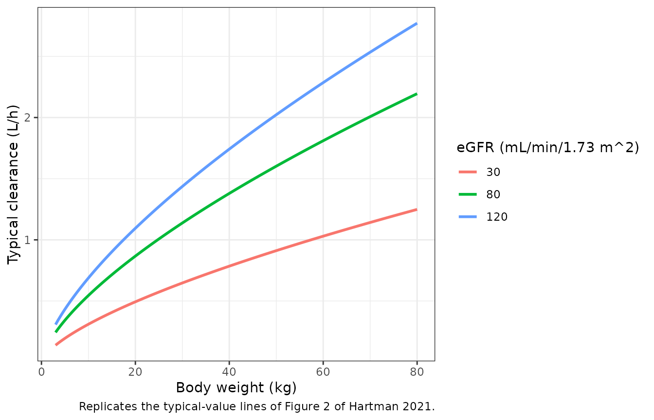

The paper reports individual clearances between 0.15 and 2.72 L/h. The typical clearance for the lightest (3.8 kg) and heaviest (75 kg) patients at the observed eGFR extremes (13.8 and 269.4 mL/min/1.73 m^2) spans 0.1 to 4.2 L/h, which brackets that range, as it must: the observed patients combine the two covariates less extremely.

Virtual cohort

The paper’s simulations resample the original 45 patients, which are not public. The virtual cohort below draws 200 children whose weight is log-normal with the observed median (14 kg) and interquartile range (8.3-32.2 kg), redrawn until it lies inside the observed range 3.8-75 kg. As in the paper’s Figure 3, eGFR and albumin are fixed at their medians (85.22 mL/min/1.73 m^2 and 27 g/L).

The random effects are drawn with base R from the model’s own OMEGA block and passed to the solver as data columns with zeroRe(). The simulation therefore uses no rxode2 random numbers and gives the same cohort on every machine. The paper computed PTA from individual-predicted troughs (Methods 2.8), so no residual error is added.

set.seed(20210526)
n_sub <- 200
omega <- rxode2::rxode2(mod)$omega
#> ℹ parameter labels from comments will be replaced by 'label()'
eta <- matrix(rnorm(2 * n_sub), n_sub, 2) %*% chol(omega)
colnames(eta) <- colnames(omega)

wt_sdlog <- (log(32.2) - log(8.3)) / (2 * qnorm(0.75))
wt <- numeric(0)
while (length(wt) < n_sub) {
  w <- exp(rnorm(n_sub, log(14), wt_sdlog))
  wt <- c(wt, w[w >= 3.8 & w <= 75])
}

cohort <- data.frame(
  id = seq_len(n_sub), WT = wt[seq_len(n_sub)], CRCL = 85.22, ALB = 27,
  etalcl = eta[, "etalcl"], etalvc = eta[, "etalvc"]
)
stopifnot(
  abs(median(cohort$WT) / 14 - 1) < 0.15,
  abs(cor(cohort$etalcl, cohort$etalvc) - 0.178 / sqrt(0.135 * 0.427)) < 0.1
)
summary(cohort$WT)
#>    Min. 1st Qu.  Median    Mean 3rd Qu.    Max. 
#>   3.927   9.340  15.280  20.937  29.004  70.483

Concentration-time profiles

regimens <- data.frame(
  regimen = c("100 mg/kg q24h", "50 mg/kg q24h", "80 mg/kg q24h", "50 mg/kg q12h"),
  dose = c(100, 50, 80, 50),
  ii = c(24, 24, 24, 12)
)

solve_regimen <- function(i, subjects, obs_times) {
  r <- regimens[i, ]
  ev <- make_events(subjects, r$dose, r$ii, 72 / r$ii, obs_times)
  ev$id <- ev$id + (i - 1L) * 1000L
  ev$regimen <- r$regimen
  withCallingHandlers(
    as.data.frame(rxode2::rxSolve(mod_typ, ev, keep = c("regimen", "WT"))),
    warning = function(w) {
      if (grepl("omega", conditionMessage(w))) invokeRestart("muffleWarning")
    }
  )
}

# 0.5-h grid, refined to 0.05 h for 2 h after each dose: the unbound peak is
# sharp because binding saturates, and PKNCA's trapezoids need the detail.
prof_times <- sort(unique(c(
  seq(0, 72, by = 0.5),
  as.vector(outer(seq(0, 2, by = 0.05), c(0, 24, 48), "+"))
)))
sim_prof <- solve_regimen(1, cohort, prof_times)
#> ℹ omega/sigma items treated as zero: 'etalcl', 'etalvc'

sim_prof |>
  dplyr::select(time, Cc, Cu) |>
  tidyr::pivot_longer(c(Cc, Cu), names_to = "analyte", values_to = "conc") |>
  dplyr::group_by(time, analyte) |>
  dplyr::summarise(
    Q05 = quantile(conc, 0.05), Q50 = median(conc), Q95 = quantile(conc, 0.95),
    .groups = "drop"
  ) |>
  dplyr::mutate(analyte = ifelse(analyte == "Cc", "Total", "Unbound")) |>
  ggplot(aes(time, Q50, colour = analyte, fill = analyte)) +
  geom_ribbon(aes(ymin = Q05, ymax = Q95), alpha = 0.2, colour = NA) +
  geom_line() +
  scale_y_log10() +
  labs(
    x = "Time (h)", y = "Ceftriaxone (mg/L)", colour = NULL, fill = NULL,
    caption = "100 mg/kg q24h, median eGFR and albumin; 5th-95th percentile band."
  ) +
  theme_bw()
#> Warning in scale_y_log10(): log-10 transformation introduced infinite values.
#> log-10 transformation introduced infinite values.
#> log-10 transformation introduced infinite values.
#> log-10 transformation introduced infinite values.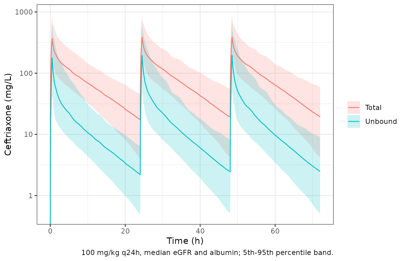

Figure 3: probability of target attainment

PTA is the percentage of children whose unbound trough concentration at 72 h exceeds the MIC (100% fT > MIC). Figure 3 reports it at the primary target of 0.5 mg/L and at 4 x MIC (2.0 mg/L) for four regimens.

troughs <- dplyr::bind_rows(lapply(seq_len(nrow(regimens)), function(i) {
  solve_regimen(i, cohort, 72)
}))
#> ℹ omega/sigma items treated as zero: 'etalcl', 'etalvc'
#> ℹ omega/sigma items treated as zero: 'etalcl', 'etalvc'
#> ℹ omega/sigma items treated as zero: 'etalcl', 'etalvc'
#> ℹ omega/sigma items treated as zero: 'etalcl', 'etalvc'
stopifnot(nrow(troughs) == 4 * n_sub, !anyNA(troughs$Cu))

mic_grid <- 2^seq(-9, 7, by = 0.25)
pta_curve <- tidyr::expand_grid(regimen = regimens$regimen, mic = mic_grid) |>
  dplyr::rowwise() |>
  dplyr::mutate(pta = 100 * mean(troughs$Cu[troughs$regimen == regimen] > mic)) |>
  dplyr::ungroup()

ggplot(pta_curve, aes(mic, pta, colour = regimen)) +
  geom_line(linewidth = 1) +
  geom_hline(yintercept = 90, linetype = "dashed") +
  geom_vline(xintercept = c(0.5, 2), colour = "grey50") +
  scale_x_log10() +
  labs(
    x = "MIC (mg/L)", y = "PTA (%)", colour = NULL,
    caption = "Replicates Figure 3 of Hartman 2021 (eGFR 85.22, albumin 27 g/L)."
  ) +
  theme_bw()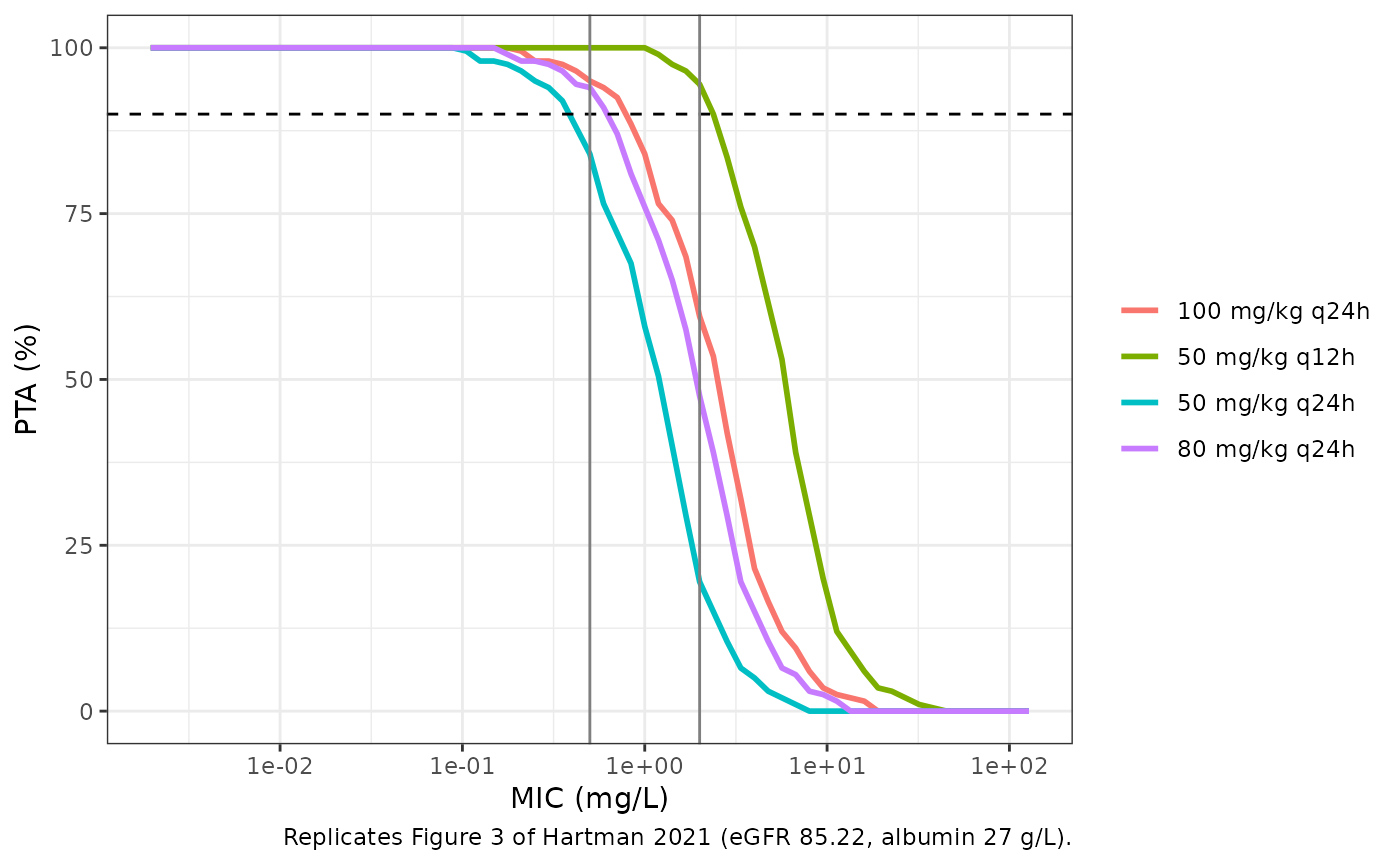

published_pta <- data.frame(
  regimen = rep(regimens$regimen, each = 2),
  mic = rep(c(0.5, 2), 4),
  paper = c(96.8, 60.8, 86.5, 29.9, 94.6, 51.3, 99.9, 93.4)
)
pta_cmp <- published_pta |>
  dplyr::rowwise() |>
  dplyr::mutate(model = 100 * mean(troughs$Cu[troughs$regimen == regimen] > mic)) |>
  dplyr::ungroup() |>
  dplyr::mutate(diff = model - paper)

pta_cmp |>
  dplyr::rename(
    "Regimen" = regimen, "MIC (mg/L)" = mic, "Paper PTA (%)" = paper,
    "Model PTA (%)" = model, "Difference (points)" = diff
  ) |>
  knitr::kable(digits = 1, caption = "PTA against the values quoted in the Results and Figure 3.")

PTA against the values quoted in the Results and Figure 3.

Regimen	MIC (mg/L)	Paper PTA (%)	Model PTA (%)	Difference (points)
100 mg/kg q24h	0.5	96.8	95.0	-1.8
100 mg/kg q24h	2.0	60.8	59.5	-1.3
50 mg/kg q24h	0.5	86.5	84.0	-2.5
50 mg/kg q24h	2.0	29.9	19.5	-10.4
80 mg/kg q24h	0.5	94.6	94.0	-0.6
80 mg/kg q24h	2.0	51.3	47.5	-3.8
50 mg/kg q12h	0.5	99.9	100.0	0.1
50 mg/kg q12h	2.0	93.4	94.5	1.1

# The cohort is deterministic (base-R draws, no rxode2 RNG), so these bounds
# do not move between machines. Measured: median |diff| 1.6 points, max 10.4
# (50 mg/kg q24h at 2 mg/L, which sits on the steepest part of its PTA
# curve). A 20% error in CL moves every 2 mg/L row by 10-20 points, so the
# median bound still catches a structural error.
stopifnot(
  median(abs(pta_cmp$diff)) < 4,
  max(abs(pta_cmp$diff)) < 12
)

The model reproduces the paper’s ranking and magnitudes: once-daily 100 mg/kg reaches more than 90% PTA only at the 0.5 mg/L target, and 50 mg/kg twice daily is the only regimen above 90% at 2 mg/L. The largest gap, about 10 points for 50 mg/kg once daily at 2 mg/L, sits on the steep part of that regimen’s PTA curve, where the weight distribution of the resampled trial patients (not available) matters most.

ESM Figure 7: PTA by eGFR and weight group

The Results state that 100 mg/kg once daily and 50 mg/kg twice daily both reach PTA above 90% for the 0.5 mg/L target in every weight group when eGFR is 80 mL/min/1.73 m^2 or lower, and that children under 10 kg with eGFR above 80 have the lowest PTA. The first claim is checked at 0.5 mg/L. The second is checked at 2 mg/L, because at 0.5 mg/L and eGFR 120 the three weight groups of a 200-child cohort differ by less than their sampling noise. The chunk below repeats the simulation with eGFR fixed at 30, 80 and 120 and the cohort split at the paper’s weight cut-offs.

strata <- dplyr::bind_rows(lapply(c(30, 80, 120), function(egfr) {
  coh <- cohort
  coh$CRCL <- egfr
  dplyr::bind_rows(lapply(c(1, 4), function(i) solve_regimen(i, coh, 72))) |>
    dplyr::mutate(CRCL = egfr)
})) |>
  dplyr::mutate(wt_group = cut(WT, c(0, 10, 25, Inf), labels = c("< 10 kg", "10-25 kg", "> 25 kg")))
#> ℹ omega/sigma items treated as zero: 'etalcl', 'etalvc'
#> ℹ omega/sigma items treated as zero: 'etalcl', 'etalvc'
#> ℹ omega/sigma items treated as zero: 'etalcl', 'etalvc'
#> ℹ omega/sigma items treated as zero: 'etalcl', 'etalvc'
#> ℹ omega/sigma items treated as zero: 'etalcl', 'etalvc'
#> ℹ omega/sigma items treated as zero: 'etalcl', 'etalvc'

pta_strata <- strata |>
  dplyr::group_by(regimen, CRCL, wt_group) |>
  dplyr::summarise(n = dplyr::n(), pta_05 = 100 * mean(Cu > 0.5), pta_2 = 100 * mean(Cu > 2), .groups = "drop")

pta_strata |>
  dplyr::rename(
    "Regimen" = regimen, "eGFR" = CRCL, "Weight group" = wt_group,
    "PTA 0.5 mg/L (%)" = pta_05, "PTA 2 mg/L (%)" = pta_2
  ) |>
  knitr::kable(digits = 1)

Regimen	eGFR	Weight group	n	PTA 0.5 mg/L (%)	PTA 2 mg/L (%)
100 mg/kg q24h	30	< 10 kg	57	100.0	94.7
100 mg/kg q24h	30	10-25 kg	86	100.0	98.8
100 mg/kg q24h	30	> 25 kg	57	100.0	98.2
100 mg/kg q24h	80	< 10 kg	57	93.0	52.6
100 mg/kg q24h	80	10-25 kg	86	97.7	61.6
100 mg/kg q24h	80	> 25 kg	57	98.2	80.7
100 mg/kg q24h	120	< 10 kg	57	84.2	15.8
100 mg/kg q24h	120	10-25 kg	86	82.6	30.2
100 mg/kg q24h	120	> 25 kg	57	89.5	49.1
50 mg/kg q12h	30	< 10 kg	57	100.0	100.0
50 mg/kg q12h	30	10-25 kg	86	100.0	100.0
50 mg/kg q12h	30	> 25 kg	57	100.0	100.0
50 mg/kg q12h	80	< 10 kg	57	100.0	91.2
50 mg/kg q12h	80	10-25 kg	86	100.0	97.7
50 mg/kg q12h	80	> 25 kg	57	100.0	98.2
50 mg/kg q12h	120	< 10 kg	57	100.0	63.2
50 mg/kg q12h	120	10-25 kg	86	100.0	80.2
50 mg/kg q12h	120	> 25 kg	57	100.0	94.7

# Measured: lowest 0.5 mg/L PTA at eGFR <= 80 is 93.0% (100 mg/kg q24h,
# < 10 kg). At eGFR 120 the three weight groups are within noise of each
# other at 0.5 mg/L (84-89%), so the "lowest PTA below 10 kg" claim is
# checked at 2 mg/L, where it is clear: 15.8 vs 30.2 vs 49.1% for
# 100 mg/kg q24h and 63.2 vs 80.2 vs 94.7% for 50 mg/kg q12h.
low_egfr <- pta_strata |> dplyr::filter(CRCL <= 80)
lowest_cell <- pta_strata |>
  dplyr::group_by(regimen) |>
  dplyr::slice_min(pta_2, n = 1, with_ties = FALSE) |>
  dplyr::ungroup()
stopifnot(
  all(low_egfr$pta_05 > 90),
  all(lowest_cell$wt_group == "< 10 kg"),
  all(lowest_cell$CRCL == 120)
)

PKNCA validation

Hartman 2021 reports no NCA parameters, so the non-compartmental check here is internal. Total-drug disposition is linear, so at steady state the AUC over one dosing interval must equal dose / CL for every child. The unbound AUC is also carried as the auc_free state (the control stream’s COMP(FREE)), which must agree with PKNCA’s trapezoidal AUC of Cu.

sim_nca <- sim_prof |>
  dplyr::filter(!is.na(Cc)) |>
  dplyr::select(id, time, Cc, Cu, regimen, cl, auc_free)

# Numerical path: tiny negative undershoots are integrator noise.
stopifnot(all(sim_nca$Cc >= -1e-6 * max(sim_nca$Cc)))

dose_df <- make_events(cohort, 100, 24, 3, numeric(0)) |>
  dplyr::filter(evid == 1) |>
  dplyr::mutate(regimen = "100 mg/kg q24h") |>
  dplyr::select(id, time, amt, regimen)

intervals <- data.frame(
  start = c(0, 48), end = c(24, 72),
  cmax = TRUE, tmax = TRUE, auclast = TRUE, cmin = TRUE
)

conc_tot <- PKNCA::PKNCAconc(sim_nca, Cc ~ time | regimen + id)
conc_unb <- PKNCA::PKNCAconc(sim_nca, Cu ~ time | regimen + id)
dose_obj <- PKNCA::PKNCAdose(dose_df, amt ~ time | regimen + id)

nca_tot <- as.data.frame(PKNCA::pk.nca(PKNCA::PKNCAdata(conc_tot, dose_obj, intervals = intervals)))
nca_unb <- as.data.frame(PKNCA::pk.nca(PKNCA::PKNCAdata(conc_unb, dose_obj, intervals = intervals)))

summarise_nca <- function(res, label) {
  res |>
    dplyr::filter(PPTESTCD %in% c("cmax", "auclast", "cmin")) |>
    dplyr::mutate(interval = ifelse(start == 0, "Day 1 (0-24 h)", "Day 3 (48-72 h)")) |>
    dplyr::group_by(interval, PPTESTCD) |>
    dplyr::summarise(median = median(PPORRES), p05 = quantile(PPORRES, 0.05), p95 = quantile(PPORRES, 0.95), .groups = "drop") |>
    dplyr::mutate(analyte = label)
}
dplyr::bind_rows(summarise_nca(nca_tot, "Total"), summarise_nca(nca_unb, "Unbound")) |>
  dplyr::rename("Analyte" = analyte, "Interval" = interval, "Parameter" = PPTESTCD, "Median" = median, "P5" = p05, "P95" = p95) |>
  dplyr::relocate(Analyte) |>
  knitr::kable(digits = 2, caption = "Simulated NCA, 100 mg/kg q24h (mg/L; AUC in mg*h/L).")

Simulated NCA, 100 mg/kg q24h (mg/L; AUC in mg*h/L).

Analyte	Interval	Parameter	Median	P5	P95
Total	Day 1 (0-24 h)	auclast	1889.49	946.42	3879.44
Total	Day 1 (0-24 h)	cmax	367.47	172.04	885.87
Total	Day 1 (0-24 h)	cmin	0.00	0.00	0.00
Total	Day 3 (48-72 h)	auclast	2139.25	1026.93	4441.24
Total	Day 3 (48-72 h)	cmax	388.35	186.02	912.16
Total	Day 3 (48-72 h)	cmin	19.18	4.17	55.33
Unbound	Day 1 (0-24 h)	auclast	419.99	168.20	1530.89
Unbound	Day 1 (0-24 h)	cmax	177.06	42.22	672.48
Unbound	Day 1 (0-24 h)	cmin	0.00	0.00	0.00
Unbound	Day 3 (48-72 h)	auclast	495.77	175.21	1616.31
Unbound	Day 3 (48-72 h)	cmax	195.30	48.63	698.43
Unbound	Day 3 (48-72 h)	cmin	2.46	0.51	8.13

# Steady-state AUC over one interval against dose / CL (individual CL).
ss_chk <- nca_tot |>
  dplyr::filter(PPTESTCD == "auclast", start == 48) |>
  dplyr::left_join(sim_nca |> dplyr::distinct(id, cl), by = "id") |>
  dplyr::left_join(cohort |> dplyr::select(id, WT), by = "id") |>
  dplyr::mutate(pct = 100 * (PPORRES * cl / (100 * WT) - 1))

# Unbound AUC from PKNCA against the auc_free state over 48-72 h.
auc_state <- sim_nca |>
  dplyr::filter(time %in% c(48, 72)) |>
  dplyr::group_by(id) |>
  dplyr::summarise(auc_state = diff(auc_free), .groups = "drop")
unb_chk <- nca_unb |>
  dplyr::filter(PPTESTCD == "auclast", start == 48) |>
  dplyr::left_join(auc_state, by = "id") |>
  dplyr::mutate(pct = 100 * (PPORRES / auc_state - 1))

# Measured: total median -0.06%, 90th percentile |pct| 0.58%, worst -5.3%
# (the slowest-clearing children are not yet at steady state by 48 h, so
# their 48-72 h AUC is still below dose / CL); unbound median 0.06%,
# 90th percentile 0.10% (trapezoid error only). A clearance or dose
# transcription error of 10% moves the total median by 10 points.
stopifnot(
  abs(median(ss_chk$pct)) < 0.5,
  quantile(abs(ss_chk$pct), 0.9) < 3,
  abs(median(unb_chk$pct)) < 0.5,
  quantile(abs(unb_chk$pct), 0.9) < 1
)

Sensitivity to BMAXpop

The control stream prints BMAXpop = 228 mg/L where Table 2 reports 223 mg/L (see Assumptions and deviations). The Figure 3 PTA is repeated with 228.

mod_typ_228 <- mod_typ |> rxode2::ini(lbmax_pb = log(228))
#> ℹ change initial estimate of `lbmax_pb` to `5.42934562895444`
troughs_228 <- dplyr::bind_rows(lapply(seq_len(nrow(regimens)), function(i) {
  r <- regimens[i, ]
  ev <- make_events(cohort, r$dose, r$ii, 72 / r$ii, 72)
  ev$id <- ev$id + (i - 1L) * 1000L
  ev$regimen <- r$regimen
  suppressWarnings(as.data.frame(rxode2::rxSolve(mod_typ_228, ev, keep = "regimen")))
}))
#> ℹ omega/sigma items treated as zero: 'etalcl', 'etalvc'
#> ℹ omega/sigma items treated as zero: 'etalcl', 'etalvc'
#> ℹ omega/sigma items treated as zero: 'etalcl', 'etalvc'
#> ℹ omega/sigma items treated as zero: 'etalcl', 'etalvc'
pta_228 <- published_pta |>
  dplyr::rowwise() |>
  dplyr::mutate(pta_228 = 100 * mean(troughs_228$Cu[troughs_228$regimen == regimen] > mic)) |>
  dplyr::ungroup()
max_shift <- max(abs(pta_228$pta_228 - pta_cmp$model))
max_shift
#> [1] 2.5
stopifnot(max_shift < 3)

Assumptions and deviations

• BMAXpop. Table 2 reports the final estimate of the maximum binding capacity as 223 mg/L; the $THETA block of the control stream printed in the ESM carries 228 mg/L. Every other stream value matches Table 2 exactly, and the table is the reported final estimate, so the model uses 223 mg/L. The choice barely matters: with 228 mg/L the Figure 3 PTA values shift by at most 2.5 percentage points (section Sensitivity to BMAXpop above).
• Weight exponent on V1. The Results text rounds it to 1.29; Table 2 and the control stream both give 1.28, which is used.
• Shared residual error. The source applies one proportional epsilon (ERR(1), variance 0.0596) to both total and unbound observations. rxode2 does not allow one parameter to serve two endpoints, so it is written twice (propSd for Cc, propSd_Cu for Cu) with the same value. Simulation is unaffected, because epsilon is drawn per observation in both programs; a re-estimation would treat the two as separate parameters.
• Omitted zero variances. The stream declares IIV on V2, Q and Kd fixed to
  0. They contribute nothing and are not carried. The ESM text says IIV on BMAX was removed at backward elimination; the stream’s remaining eta sits on Kd and is fixed to 0 either way.
• eGFR covariate. Clearance uses each patient’s median creatinine-based eGFR over the study period (stream column EGFR_KREAT_patmedian), not the time-varying value, so CRCL should be supplied as one value per child. The stream’s eGFR is Schwartz 2012, 42.3 x (height / SCr in mg/dL)^0.79. The authors advise caution above 120 mL/min/1.73 m^2 in children over 25 kg.
• Missing albumin. The source coded a missing albumin as 0 and reset its effect to 1 (IF (ALBUMIN.EQ.0) COV_ALB_FU = 1). That data-coding branch is not reproduced; supply 27 g/L for a child without an albumin value to get the same behaviour.
• Unbound AUC state. The stream’s third compartment accumulates the unbound concentration. It is kept as auc_free and feeds nothing else.
• Virtual cohort. The paper resampled its own 45 patients; this vignette uses a log-normal weight distribution matched to the reported median and IQR. No maximum-dose cap (2 g prophylactic, 4 g therapeutic per day) is applied, because the Methods do not say one was applied in the simulations.
• No erratum or correction notice for Hartman 2021 was found in PubMed or Crossref as of 2026-09-29.