Thrombomodulin alfa (Mouksassi 2015)

Model and source

• Citation: Mouksassi MS, Marier JF, Bax L, Osawa Y, Tsuruta K. (2015). Population Pharmacokinetic Analysis of Thrombomodulin Alfa to Support Dosing Rationale in Patients with Renal Impairment. Clin Pharmacol Drug Dev. 4(3):210-217. doi:10.1002/cpdd.163
• Description: One-compartment intravenous population PK model for thrombomodulin alfa (ART-123, a soluble recombinant human thrombomodulin) pooled across 24 healthy adults given single 0.02 or 0.06 mg/kg IV doses and 368 adults with sepsis and suspected disseminated intravascular coagulation given 0.06 mg/kg/day (maximum 6 mg) IV for six consecutive days (Mouksassi 2015; N = 392). Typical clearance is 0.14 L/h and typical central volume 5.47 L at the reference 68 kg body weight and 72.6 mL/min creatinine clearance, giving a typical elimination half-life of 27.08 h. Clearance carries a power effect of body weight (exponent 0.56) and of baseline Cockcroft-Gault creatinine clearance truncated at 150 mL/min (exponent 0.27); central volume carries a power effect of body weight (exponent 0.50). Between-subject variability is log-normal on clearance (variance 0.11, i.e. 33% on the SD scale) and on central volume (variance 0.15, i.e. 39%), correlated at 0.57. Residual variability is proportional (29%). The analysis supports the conclusion that no dose adjustment is needed in sepsis and DIC patients with mild to severe renal impairment, because simulated exposures stay inside the 300-5400 ng/mL therapeutic range.
• Article: https://doi.org/10.1002/cpdd.163

Thrombomodulin alfa (ART-123) is a soluble recombinant human thrombomodulin developed for disseminated intravascular coagulation (DIC) in sepsis. Because the drug is cleared predominantly renally and because its principal safety concern is bleeding driven by high plasma concentrations, the purpose of the population PK analysis was to decide whether renally impaired patients need a dose reduction. The paper’s answer is no: over the range of renal function studied, simulated exposures stay inside the 300-5400 ng/mL therapeutic range.

The structural model is one-compartment with linear elimination:

$$\frac{\mathrm{d}A_\mathrm{central}}{\mathrm{d}t} = -\frac{CL}{V}\,A_\mathrm{central}, \qquad C_c = 1000\times\frac{A_\mathrm{central}}{V}$$

$$CL = 0.14 \left(\frac{WT}{68}\right)^{0.56}\left(\frac{CRCL}{72.6}\right)^{0.27} \ \mathrm{L/h}, \qquad V = 5.47 \left(\frac{WT}{68}\right)^{0.50}\ \mathrm{L}$$

Population

The analysis pooled two studies (N = 392). The first was a Phase I single-dose trial of 0.02 and 0.06 mg/kg intravenous ART-123 in 24 normal healthy volunteers with rich sampling (baseline; 5, 10, 15, 30 min; 1, 2, 4, 6, 8, 12, 24, 36, 48, 72, 96, 120 and 144 h). The second was a randomised, double-blind, placebo-controlled Phase IIb study in patients with sepsis and suspected DIC; the 368 ART-123-treated subjects who provided plasma samples were included, sampled sparsely (12 +/- 3 h after the Day 1 dose, within 30 min before the Day 3 dose, 12 +/- 3 h after the Day 3 dose, Day 7, Day 14 and in some cases Day 28). Phase IIb dosing was 0.06 mg/kg/day up to a maximum of 6 mg once daily for six consecutive days, given as an IV bolus or a 15-minute IV infusion.

Combined baseline characteristics (Mouksassi 2015 Table 1) were mean age 55.8 years (range 18-93), mean weight 70.54 kg (median 68, range 30-150) and mean creatinine clearance 74.6 mL/min (range 5-150). Renal function differed sharply between the two studies – Phase I mean CrCL 114.2 mL/min versus Phase IIb 72.0 mL/min – which is what makes the pooled dataset informative about renal impairment. Patients receiving renal replacement therapy for end-stage renal disease or acute kidney injury were excluded, so the model is not qualified for dialysis or ESRD. Sex and race are reported over 380 rather than 392 subjects (142 female / 238 male; 62.1% Caucasian, 26.1% Indian, 5.8% Asian, 3.4% Black, 2.4% Other, 0.3% Hispanic); the paper does not explain the difference.

The same information is available programmatically via the model’s population metadata (readModelDb("Mouksassi_2015_thrombomodulinAlfa")()$population).

Source trace

The per-parameter origin is recorded as an in-file comment next to each ini() entry in inst/modeldb/specificDrugs/Mouksassi_2015_thrombomodulinAlfa.R. The table below collects them in one place for review.

Equation / parameter	Value	Source location
lcl (CL at WT 68 kg, CRCL 72.6 mL/min)	0.14 L/h (2.01% SE)	Table 2, CL row
lvc (V at WT 68 kg)	5.47 L (2.71% SE)	Table 2, V row
e_wt_cl	0.56 (14.15% SE)	Table 2, CL row exponent; added at Table S2 step 1
e_crcl_cl	0.27 (12.56% SE)	Table 2, CL row exponent; added at Table S2 step 2
e_wt_vc	0.50 (21.14% SE)	Table 2, V row exponent; added at Table S2 step 3
etalcl variance	0.11 (10.59% SE)	Table 2, BSV column; scale confirmed by Figure 3A (“BSV = 33 %”, = sqrt(0.11))
etalvc variance	0.15 (14.21% SE)	Table 2, BSV column; scale confirmed by Figure 3B (“BSV = 39 %”, = sqrt(0.15))
etalcl/etalvc covariance	0.0732	Table 2 footnote a, reconstructed from the printed correlation 0.57 (see Errata)
propSd	0.29 (2.43% SE)	Table 2, “Proportional error” row
Reference body weight	68 kg	Table 2 equations; equals the Table 1 combined median weight
Reference creatinine clearance	72.6 mL/min	Table 2 CL equation; independently confirmed by the Figure 3A CrCL bar (see below)
Covariate model as a whole	8 annotated values	Figure 3 Panels A and B, each reproduced exactly at the printed precision
CRCL truncation at 150 mL/min	n/a	Results, “Demographics and Baseline Characteristics”
One-compartment structure, proportional error	n/a	Results paragraph 1 and Supplemental Table S1 (AIC 22,618, vs 22,624 mixed error and 23,645 additive error; the two-compartment model is lower on AIC at 22,607 but higher on BIC – see Errata)
d/dt(central), Cc	n/a	Methods, “Population PK Modeling”; concentration unit ng/mL per Bioanalytical Assay and Figure 4 y-axis

Renal-function strata

The paper’s dosing-rationale simulations use four renal-function strata defined by Cockcroft-Gault creatinine clearance, each represented by the median of its range.

strata <- tibble::tribble(
  ~stratum,   ~crcl_med, ~crcl_lo, ~crcl_hi, ~cl_pub, ~v_pub, ~thalf_pub,
  "Normal",     105,       90,      120,      0.158,   5.44,   NA_real_,
  "Mild",        75,       60,       89,      0.145,   5.48,   26.2,
  "Moderate",    45,       30,       59,      0.128,   5.54,   30.0,
  "Severe",      22,       15,       30,      0.105,   5.45,   36.0
) |>
  dplyr::mutate(stratum = factor(stratum, levels = c("Normal", "Mild", "Moderate", "Severe")))

knitr::kable(
  strata |>
    dplyr::rename(
      "Renal function"         = stratum,
      "CrCL median (mL/min)"   = crcl_med,
      "CrCL low (mL/min)"      = crcl_lo,
      "CrCL high (mL/min)"     = crcl_hi,
      "Published CL (L/h)"     = cl_pub,
      "Published V (L)"        = v_pub,
      "Published t1/2 (h)"     = thalf_pub
    ),
  caption = paste(
    "Renal-function strata and the typical parameter values Mouksassi 2015",
    "reports for each (Results, 'Final Population PK Model'). The paper prints",
    "t1/2 only for the three impairment strata."
  )
)

Renal-function strata and the typical parameter values Mouksassi 2015 reports for each (Results, ‘Final Population PK Model’). The paper prints t1/2 only for the three impairment strata.

Renal function	CrCL median (mL/min)	CrCL low (mL/min)	CrCL high (mL/min)	Published CL (L/h)	Published V (L)	Published t1/2 (h)
Normal	105	90	120	0.158	5.44	NA
Mild	75	60	89	0.145	5.48	26.2
Moderate	45	30	59	0.128	5.54	30.0
Severe	22	15	30	0.105	5.45	36.0

The published stratum values are internally consistent: t1/2 = ln(2) * V / CL recovers each printed half-life from the printed CL and V of the same stratum.

thalf_from_pub <- log(2) * strata$v_pub / strata$cl_pub
stopifnot(
  # Reproduces 26.2, 30.0 and 36.0 h to the printed precision.
  max(abs(thalf_from_pub - strata$thalf_pub), na.rm = TRUE) < 0.05
)
round(thalf_from_pub, 2)
#> [1] 23.87 26.20 30.00 35.98

Note that the published stratum volumes (5.44-5.54 L) differ slightly from the reference 5.47 L because each stratum’s median body weight differs slightly from 68 kg; the model itself has no CrCL effect on volume.

Typical-value parameters and the reference half-life

The single tightest check on the transcription is the reference subject: at WT = 68 kg and CRCL = 72.6 mL/min the covariate terms are both exactly 1, so CL must be 0.14 L/h, V must be 5.47 L, and the half-life must be the 27.08 h printed in Table 2.

mod <- readModelDb("Mouksassi_2015_thrombomodulinAlfa")
mod_typ <- rxode2::zeroRe(mod)
#> ℹ parameter labels from comments will be replaced by 'label()'

# One subject per arm is enough with the random effects zeroed out.
ref_ev <- data.frame(
  id   = 1L,
  time = c(0, 0.25),
  amt  = c(0.06 * 68, 0),
  rate = c(0.06 * 68 / 0.25, 0),
  evid = c(1L, 0L),
  cmt  = "central",
  WT   = 68,
  CRCL = 72.6
)

ref_sim <- rxode2::rxSolve(mod_typ, ref_ev, omega = NA, returnType = "data.frame")
ref_cl <- ref_sim$cl[1]
ref_vc <- ref_sim$vc[1]
ref_thalf <- log(2) * ref_vc / ref_cl

stopifnot(
  abs(ref_cl - 0.14) < 1e-8,
  abs(ref_vc - 5.47) < 1e-8,
  # Table 2 prints 27.08 h and its footnote defines t1/2 = Ln(2)/(CL/V).
  abs(ref_thalf - 27.08) < 0.01
)
c(CL = ref_cl, V = ref_vc, t_half = ref_thalf)
#>       CL        V   t_half 
#>  0.14000  5.47000 27.08225

Evaluating the same equations across the four strata at the reference weight gives the model’s typical values, which can be put next to the paper’s.

typ_ev <- strata |>
  dplyr::transmute(stratum = as.character(stratum), CRCL = crcl_med, WT = 68) |>
  dplyr::mutate(id = dplyr::row_number()) |>
  tidyr::crossing(time = c(0, 0.25)) |>
  dplyr::mutate(
    amt  = ifelse(time == 0, 0.06 * WT, 0),
    rate = ifelse(time == 0, 0.06 * WT / 0.25, 0),
    evid = ifelse(time == 0, 1L, 0L),
    cmt  = "central"
  ) |>
  dplyr::arrange(id, time, dplyr::desc(evid))

typ_sim <- rxode2::rxSolve(mod_typ, typ_ev, omega = NA,
                           keep = "stratum", returnType = "data.frame")
#> Warning: multi-subject simulation without without 'omega'

typ_par <- typ_sim |>
  dplyr::mutate(stratum = as.character(stratum)) |>
  dplyr::group_by(stratum) |>
  dplyr::summarise(cl_mod = dplyr::first(cl), v_mod = dplyr::first(vc), .groups = "drop") |>
  dplyr::mutate(thalf_mod = log(2) * v_mod / cl_mod) |>
  dplyr::left_join(
    strata |> dplyr::transmute(stratum = as.character(stratum), cl_pub, v_pub, thalf_pub),
    by = "stratum"
  ) |>
  dplyr::mutate(
    stratum = factor(stratum, levels = levels(strata$stratum))
  ) |>
  dplyr::arrange(stratum) |>
  dplyr::mutate(
    cl_pct    = 100 * (cl_mod - cl_pub) / cl_pub,
    thalf_pct = 100 * (thalf_mod - thalf_pub) / thalf_pub
  )

knitr::kable(
  typ_par |>
    dplyr::rename(
      "Renal function"    = stratum,
      "CL model (L/h)"    = cl_mod,
      "V model (L)"       = v_mod,
      "t1/2 model (h)"    = thalf_mod,
      "CL published (L/h)" = cl_pub,
      "V published (L)"   = v_pub,
      "t1/2 published (h)" = thalf_pub,
      "CL % diff"         = cl_pct,
      "t1/2 % diff"       = thalf_pct
    ),
  digits = c(0, 4, 3, 2, 4, 3, 2, 1, 1),
  caption = paste(
    "Model typical values at WT = 68 kg versus the values Mouksassi 2015",
    "reports for each renal-function stratum."
  )
)

Model typical values at WT = 68 kg versus the values Mouksassi 2015 reports for each renal-function stratum.

Renal function	CL model (L/h)	V model (L)	t1/2 model (h)	CL published (L/h)	V published (L)	t1/2 published (h)	CL % diff	t1/2 % diff
Normal	0.1547	5.47	24.51	0.158	5.44	NA	-2.1	NA
Mild	0.1412	5.47	26.85	0.145	5.48	26.2	-2.6	2.5
Moderate	0.1230	5.47	30.82	0.128	5.54	30.0	-3.9	2.7
Severe	0.1014	5.47	37.38	0.105	5.45	36.0	-3.4	3.8

The model runs about 2-4% below the paper’s stratum clearances (and therefore 2-4% above its half-lives) throughout. The offset is constant in sign and magnitude across all four strata, which is the signature of a rounding difference in the single multiplicative constant rather than a mis-transcribed exponent or normaliser: Table 2 prints the typical CL to two significant figures (“0.14”), and a true value of about 0.1437 – well inside that rounding interval – reconciles every stratum. See Errata.

stopifnot(
  # Structural: a wrong exponent, normaliser or unit moves individual strata by
  # tens of percent and breaks the constant-offset pattern immediately.
  max(abs(typ_par$cl_pct)) < 6,
  max(abs(typ_par$thalf_pct), na.rm = TRUE) < 6,
  # The offset is a single constant, not a covariate-shape error: the spread of
  # the per-stratum CL deviations is small compared with the deviations.
  diff(range(typ_par$cl_pct)) < 3
)

Replicating Figure 3

Figure 3 is the tightest gate in the paper on the transcription of the covariate model, and it is free: each panel is a tornado plot that prints the typical parameter value together with the parameter evaluated at the extreme of each covariate. Panel A gives clearance at the lowest and highest observed creatinine clearance (5.29 and 150 mL/min) and at the lowest and highest observed body weight (30 and 150 kg); Panel B gives volume at the two weight extremes. Eight printed numbers in all, every one of them an exact consequence of the Table 2 equations – so they pin both exponents on clearance, the exponent on volume, both typical values, and, critically, the 72.6 mL/min creatinine-clearance reference, which is the one constant in Table 2 that is not recoverable from Table 1.

fig3_cases <- tibble::tribble(
  ~panel, ~case,            ~WT,  ~CRCL,
  "A",    "Typical CL/F",    68,   72.6,
  "A",    "CRCL 5.29 mL/min", 68,   5.29,
  "A",    "CRCL 150 mL/min", 68,  150,
  "A",    "WT 30 kg",        30,   72.6,
  "A",    "WT 150 kg",      150,   72.6
) |>
  dplyr::mutate(id = dplyr::row_number())

fig3_ev <- fig3_cases |>
  tidyr::crossing(time = c(0, 0.25)) |>
  dplyr::mutate(
    amt  = ifelse(time == 0, 1, 0),
    evid = ifelse(time == 0, 1L, 0L),
    cmt  = "central"
  ) |>
  dplyr::arrange(id, time, dplyr::desc(evid))

fig3_par <- rxode2::rxSolve(mod_typ, fig3_ev, omega = NA, keep = "case",
                            returnType = "data.frame") |>
  dplyr::group_by(case) |>
  dplyr::summarise(cl = dplyr::first(cl), vc = dplyr::first(vc), .groups = "drop")
#> Warning: multi-subject simulation without without 'omega'

getpar <- function(case, what) fig3_par[[what]][match(case, fig3_par$case)]

# Panel A prints clearance to two decimal places, Panel B volume to two decimal
# places. Every printed value is reproduced EXACTLY at that precision, so the
# assertion is equality after rounding rather than a tolerance band -- the
# strictest form this check can take.
stopifnot(
  round(getpar("Typical CL/F",      "cl"), 2) == 0.14,   # Fig 3A, "0.14"
  round(getpar("CRCL 5.29 mL/min",  "cl"), 2) == 0.07,   # Fig 3A, left  of the CRCL bar
  round(getpar("CRCL 150 mL/min",   "cl"), 2) == 0.17,   # Fig 3A, right of the CRCL bar
  round(getpar("WT 30 kg",          "cl"), 2) == 0.09,   # Fig 3A, left  of the WT bar
  round(getpar("WT 150 kg",         "cl"), 2) == 0.22,   # Fig 3A, right of the WT bar
  round(getpar("Typical CL/F",      "vc"), 2) == 5.47,   # Fig 3B, "5.47"
  round(getpar("WT 30 kg",          "vc"), 2) == 3.63,   # Fig 3B, left  of the WT bar
  round(getpar("WT 150 kg",         "vc"), 2) == 8.12    # Fig 3B, right of the WT bar
)

knitr::kable(
  tibble::tribble(
    ~panel, ~quantity,  ~case,               ~published,
    "A",    "CL (L/h)", "Typical CL/F",      0.14,
    "A",    "CL (L/h)", "CRCL 5.29 mL/min",  0.07,
    "A",    "CL (L/h)", "CRCL 150 mL/min",   0.17,
    "A",    "CL (L/h)", "WT 30 kg",          0.09,
    "A",    "CL (L/h)", "WT 150 kg",         0.22,
    "B",    "V (L)",    "Typical V/F",       5.47,
    "B",    "V (L)",    "WT 30 kg",          3.63,
    "B",    "V (L)",    "WT 150 kg",         8.12
  ) |>
    dplyr::mutate(
      model = ifelse(
        quantity == "CL (L/h)",
        getpar(case, "cl"),
        getpar(ifelse(case == "Typical V/F", "Typical CL/F", case), "vc")
      ),
      rounded = round(model, 2)
    ) |>
    dplyr::rename(
      "Figure 3 panel" = panel,
      "Quantity"       = quantity,
      "Covariate case" = case,
      "Published"      = published,
      "Model"          = model,
      "Model rounded"  = rounded
    ),
  digits = c(0, 0, 0, 2, 4, 2),
  caption = paste(
    "Every value annotated on Figure 3 of Mouksassi 2015, reproduced from the",
    "model. Panel B has no CrCL bar because volume carries no creatinine",
    "clearance effect."
  )
)

Every value annotated on Figure 3 of Mouksassi 2015, reproduced from the model. Panel B has no CrCL bar because volume carries no creatinine clearance effect.

Figure 3 panel	Quantity	Covariate case	Published	Model	Model rounded
A	CL (L/h)	Typical CL/F	0.14	0.1400	0.14
A	CL (L/h)	CRCL 5.29 mL/min	0.07	0.0690	0.07
A	CL (L/h)	CRCL 150 mL/min	0.17	0.1703	0.17
A	CL (L/h)	WT 30 kg	0.09	0.0885	0.09
A	CL (L/h)	WT 150 kg	0.22	0.2180	0.22
B	V (L)	Typical V/F	5.47	5.4700	5.47
B	V (L)	WT 30 kg	3.63	3.6332	3.63
B	V (L)	WT 150 kg	8.12	8.1242	8.12

Because volume does not depend on creatinine clearance, Panel B has only a weight bar – which is itself a check: a stray CrCL term on vc would be invisible in the stratum comparison above (where the published volumes vary only 2%) but would break Panel B immediately.

Replicating Figure 4

Figure 4 of Mouksassi 2015 shows typical-value concentration-time profiles for the four renal-function strata over six consecutive daily 0.06 mg/kg doses, followed by washout out to 264 h. The two claims made from it are that the minimum concentration after the first dose exceeds the 300 ng/mL effective concentration in every stratum, and that the maximum concentration after the last dose stays below the 5400 ng/mL bleeding-risk threshold in every stratum.

make_daily_events <- function(id, wt, crcl, stratum, obs_times) {
  dose_amt <- min(0.06 * wt, 6)  # Phase IIb capped daily dose at 6 mg
  dose_times <- seq(0, by = 24, length.out = 6)
  dplyr::bind_rows(
    data.frame(time = dose_times, amt = dose_amt, rate = dose_amt / 0.25, evid = 1L),
    data.frame(time = obs_times, amt = 0, rate = 0, evid = 0L)
  ) |>
    dplyr::mutate(id = id, cmt = "central", WT = wt, CRCL = crcl, stratum = stratum) |>
    dplyr::arrange(time, dplyr::desc(evid))
}

obs_grid <- sort(unique(c(seq(0, 264, by = 0.5), seq(0, by = 24, length.out = 6) + 0.25)))

fig4_ev <- do.call(
  dplyr::bind_rows,
  lapply(seq_len(nrow(strata)), function(i) {
    make_daily_events(i, 68, strata$crcl_med[i], as.character(strata$stratum[i]), obs_grid)
  })
)
# Assert on the frame itself, NOT on unique() of it: `!anyDuplicated(unique(x))`
# is vacuously TRUE and would never catch a collision.
stopifnot(!anyDuplicated(fig4_ev[, c("id", "time", "evid")]))

fig4 <- rxode2::rxSolve(mod_typ, fig4_ev, omega = NA,
                        keep = "stratum", returnType = "data.frame") |>
  dplyr::mutate(stratum = factor(stratum, levels = levels(strata$stratum)))
#> Warning: multi-subject simulation without without 'omega'

# Replicates Figure 4 of Mouksassi 2015: typical-value profiles by renal stratum.
ggplot(fig4, aes(time, Cc, colour = stratum)) +
  geom_line(linewidth = 0.7) +
  geom_hline(yintercept = c(300, 5400), linetype = "dashed", colour = "grey40") +
  scale_x_continuous(breaks = seq(0, 264, by = 24)) +
  labs(
    x = "Time (h)", y = "Predicted concentration (ng/mL)", colour = "Renal function",
    title = "Figure 4 - predicted profiles by renal function",
    caption = paste(
      "Replicates Figure 4 of Mouksassi 2015 (0.06 mg/kg/day for six days,",
      "WT = 68 kg). Dashed lines are the 300-5400 ng/mL therapeutic range."
    )
  ) +
  theme_bw()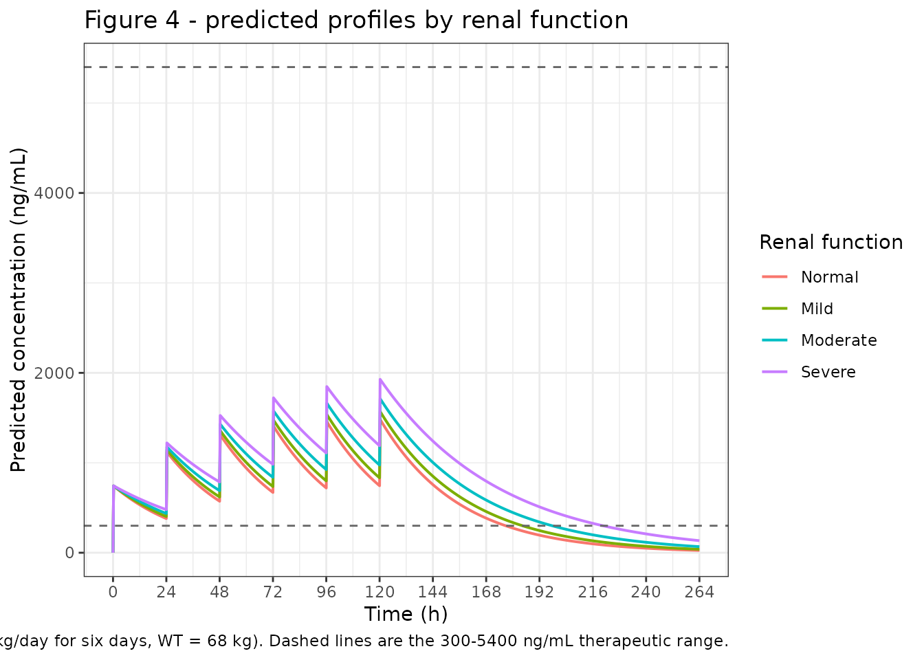

# rxSolve returns observation rows only and carries no `evid` column, so no
# filtering is needed (and filtering on evid would error).
fig4_claims <- fig4 |>
  dplyr::group_by(stratum) |>
  dplyr::summarise(
    cmax_first = max(Cc[time <= 24]),
    cmin_first = Cc[which.min(abs(time - 24))],
    cmax_last  = max(Cc[time >= 120 & time <= 144]),
    .groups    = "drop"
  )

knitr::kable(
  fig4_claims |>
    dplyr::rename(
      "Renal function"                = stratum,
      "Cmax after 1st dose (ng/mL)"   = cmax_first,
      "Cmin after 1st dose (ng/mL)"   = cmin_first,
      "Cmax after last dose (ng/mL)"  = cmax_last
    ),
  digits = 0,
  caption = paste(
    "Therapeutic-range claims of Mouksassi 2015: minimum concentration after",
    "the first dose above 300 ng/mL, maximum concentration after the last dose",
    "below 5400 ng/mL, in every renal-function stratum."
  )
)

Therapeutic-range claims of Mouksassi 2015: minimum concentration after the first dose above 300 ng/mL, maximum concentration after the last dose below 5400 ng/mL, in every renal-function stratum.

Renal function	Cmax after 1st dose (ng/mL)	Cmin after 1st dose (ng/mL)	Cmax after last dose (ng/mL)
Normal	743	380	1483
Mild	743	403	1571
Moderate	744	436	1713
Severe	744	479	1928

stopifnot(
  # The paper's two explicit claims, reproduced as written.
  all(fig4_claims$cmin_first > 300),
  all(fig4_claims$cmax_last < 5400),
  # Peak after the first dose is set by V alone, which carries no CrCL effect,
  # so it must be essentially identical across strata (only the small amount
  # eliminated during the 15-minute infusion differs).
  max(fig4_claims$cmax_first) / min(fig4_claims$cmax_first) < 1.01,
  # Figure 4's first peak reads about 750 ng/mL: 0.06 * 68 mg into 5.47 L.
  abs(max(fig4_claims$cmax_first) - 1000 * 0.06 * 68 / 5.47) / (1000 * 0.06 * 68 / 5.47) < 0.01
)

The simulated first peak is 744 ng/mL and the highest peak after the sixth dose is 1928 ng/mL, against a Figure 4 y-axis that tops out just below 2000 ng/mL.

Virtual cohort and variability

The published figure is a typical-value prediction. Adding the between-subject variability shows the spread the model actually implies, which is what matters for the bleeding-risk argument.

# Two independent RNG streams are in play and BOTH must be seeded: base R draws
# the covariates (weight, CrCL) and rxode2 draws the etas inside rxSolve().
# set.seed() alone does not fix the eta draws.
set.seed(20260826)
rxode2::rxSetSeed(20260826)

n_per_arm <- 200L

# Body weight approximating the Phase IIb distribution (mean 70.30 kg,
# SD 19.397, range 30-150; Mouksassi 2015 Table 1), drawn as a log-normal
# matched on mean and SD then truncated to the observed range.
draw_weight <- function(n) {
  m <- 70.30; s <- 19.397
  mu <- log(m^2 / sqrt(s^2 + m^2))
  sd <- sqrt(log(1 + s^2 / m^2))
  wt <- numeric(0)
  while (length(wt) < n) {
    cand <- stats::rlnorm(2 * n, mu, sd)
    wt <- c(wt, cand[cand >= 30 & cand <= 150])
  }
  wt[seq_len(n)]
}

cohort_ev <- do.call(
  dplyr::bind_rows,
  lapply(seq_len(nrow(strata)), function(i) {
    ids <- (i - 1L) * n_per_arm + seq_len(n_per_arm)
    wt <- draw_weight(n_per_arm)
    # CrCL uniform within the stratum's published range.
    crcl <- stats::runif(n_per_arm, strata$crcl_lo[i], strata$crcl_hi[i])
    do.call(
      dplyr::bind_rows,
      lapply(seq_len(n_per_arm), function(j) {
        make_daily_events(ids[j], wt[j], crcl[j], as.character(strata$stratum[i]),
                          seq(0, 264, by = 4))
      })
    )
  })
) |>
  # Carried through rxSolve() via keep= so that downstream joins key on a
  # subject id rxode2 cannot renumber. unname() because keep= rejects a named
  # column.
  dplyr::mutate(subjid = unname(id))

stopifnot(
  !anyDuplicated(cohort_ev[, c("id", "time", "evid")]),
  nrow(dplyr::distinct(cohort_ev, id)) == n_per_arm * nrow(strata)
)

# rxSolve() on an rxUi scales super-linearly in subjects per call, so solve one
# stratum (200 subjects) per call rather than all 800 at once. The RNG stream is
# seeded once above and consumed in a deterministic arm order, so batching does
# not cost reproducibility.
cohort_sim <- do.call(
  dplyr::bind_rows,
  lapply(levels(strata$stratum), function(s) {
    rxode2::rxSolve(
      mod,
      dplyr::filter(cohort_ev, stratum == s),
      keep        = c("stratum", "subjid"),
      returnType  = "data.frame"
    )
  })
) |>
  dplyr::mutate(stratum = factor(stratum, levels = levels(strata$stratum)))
#> ℹ parameter labels from comments will be replaced by 'label()'

stopifnot(
  # Batching must not lose or duplicate subjects.
  dplyr::n_distinct(cohort_sim$subjid) == n_per_arm * nrow(strata)
)

cohort_sim |>
  dplyr::group_by(stratum, time) |>
  dplyr::summarise(
    Q05 = quantile(Cc, 0.05), Q50 = median(Cc), Q95 = quantile(Cc, 0.95),
    .groups = "drop"
  ) |>
  ggplot(aes(time, Q50)) +
  geom_ribbon(aes(ymin = Q05, ymax = Q95), alpha = 0.25, fill = "steelblue") +
  geom_line(colour = "steelblue4") +
  geom_hline(yintercept = c(300, 5400), linetype = "dashed", colour = "grey40") +
  facet_wrap(~stratum) +
  scale_y_log10() +
  labs(
    x = "Time (h)", y = "Cc (ng/mL)",
    title = "Simulated variability by renal-function stratum",
    caption = paste0(
      "Median and 5th-95th percentile of ", n_per_arm, " subjects per stratum, ",
      "0.06 mg/kg/day (capped at 6 mg) for six days. Dashed lines are the ",
      "300-5400 ng/mL therapeutic range."
    )
  ) +
  theme_bw()
#> Warning in scale_y_log10(): log-10 transformation introduced infinite values.
#> log-10 transformation introduced infinite values.
#> log-10 transformation introduced infinite values.
#> log-10 transformation introduced infinite values.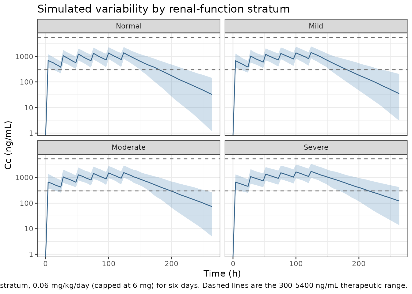

cohort_peak <- cohort_sim |>
  dplyr::group_by(stratum, subjid) |>
  dplyr::summarise(cmax_overall = max(Cc), .groups = "drop")

pct_over <- 100 * mean(cohort_peak$cmax_overall > 5400)

stopifnot(
  # The paper's conclusion is about the population, not one typical subject:
  # even with full between-subject variability the upper safety bound is not
  # approached. Asserted on robust quantiles, never on the cohort extreme,
  # which is not reproducible across rxode2 versions.
  quantile(cohort_peak$cmax_overall, 0.95) < 5400,
  # The median peak is well inside the range in every stratum.
  all(tapply(cohort_peak$cmax_overall, cohort_peak$stratum, median) < 3000)
)
sprintf(
  "median peak %.0f ng/mL, 95th percentile %.0f ng/mL, %.1f%% of subjects above 5400 ng/mL",
  median(cohort_peak$cmax_overall),
  quantile(cohort_peak$cmax_overall, 0.95),
  pct_over
)
#> [1] "median peak 1511 ng/mL, 95th percentile 2793 ng/mL, 0.0% of subjects above 5400 ng/mL"

Structural identities

These checks compare the simulation against closed-form consequences of the same drawn parameters, so they are exact up to solver tolerance and are asserted tightly.

# Per-subject covariates come from the event table (one row per subject) and
# the realised individual parameters from the solve (one row per subject). Both
# sides are per-subject and keyed on subjid, so the join is one-to-one and
# cannot fan out.
subj_cov <- cohort_ev |>
  dplyr::distinct(subjid, WT, CRCL, stratum)

subj_par <- cohort_sim |>
  dplyr::group_by(subjid) |>
  dplyr::summarise(cl = dplyr::first(cl), vc = dplyr::first(vc), .groups = "drop") |>
  dplyr::inner_join(subj_cov, by = "subjid")

stopifnot(nrow(subj_par) == n_per_arm * nrow(strata))

# The model equations, re-evaluated outside rxode2 from the covariates and the
# realised individual parameters, must reproduce the covariate terms exactly.
implied_cl_ratio <- subj_par$cl /
  ((subj_par$WT / 68)^0.56 * (subj_par$CRCL / 72.6)^0.27)
implied_vc_ratio <- subj_par$vc / (subj_par$WT / 68)^0.50

stopifnot(
  # exp(lcl + etalcl) and exp(lvc + etalvc) are the only remaining factors, so
  # the geometric mean of these ratios must sit at the typical values 0.14/5.47.
  abs(exp(mean(log(implied_cl_ratio))) - 0.14) / 0.14 < 0.05,
  abs(exp(mean(log(implied_vc_ratio))) - 5.47) / 5.47 < 0.05,
  # Realised between-subject SDs must match the published omegas
  # sqrt(0.11) = 0.332 and sqrt(0.15) = 0.387.
  abs(sd(log(implied_cl_ratio)) - sqrt(0.11)) < 0.05,
  abs(sd(log(implied_vc_ratio)) - sqrt(0.15)) < 0.05,
  # ... and so must the correlation, 0.57 as reconstructed from Table 2.
  abs(cor(log(implied_cl_ratio), log(implied_vc_ratio)) - 0.57) < 0.10
)

c(
  omega_cl_sd = sd(log(implied_cl_ratio)),
  omega_vc_sd = sd(log(implied_vc_ratio)),
  correlation = cor(log(implied_cl_ratio), log(implied_vc_ratio))
)
#> omega_cl_sd omega_vc_sd correlation 
#>   0.3404846   0.3985524   0.6069469

PKNCA validation

A single 0.06 mg/kg dose at the reference weight, one typical subject per stratum, sampled densely enough to characterise the terminal phase. Because the profile after the infusion is mono-exponential, PKNCA’s lin-up/log-down AUC and its terminal-slope half-life recover the model’s own Dose/CL and ln(2) * V / CL exactly; any difference from the published values is therefore attributable to the paper, not to the NCA.

nca_times <- sort(unique(c(
  0, seq(0, 0.25, by = 1 / 24), 0.5, 0.75, 1, 1.5, 2, 3, 4, 6, 8, 12,
  seq(18, 336, by = 6)
)))

nca_ev <- do.call(
  dplyr::bind_rows,
  lapply(seq_len(nrow(strata)), function(i) {
    dose_amt <- 0.06 * 68
    dplyr::bind_rows(
      data.frame(time = 0, amt = dose_amt, rate = dose_amt / 0.25, evid = 1L),
      data.frame(time = nca_times, amt = 0, rate = 0, evid = 0L)
    ) |>
      dplyr::mutate(id = i, cmt = "central", WT = 68, CRCL = strata$crcl_med[i],
                    stratum = as.character(strata$stratum[i])) |>
      dplyr::arrange(time, dplyr::desc(evid))
  })
)

nca_sim <- rxode2::rxSolve(mod_typ, nca_ev, omega = NA, keep = "stratum",
                           returnType = "data.frame")
#> Warning: multi-subject simulation without without 'omega'

# Keep the time-zero anchor (Cc = 0 before a 15-minute infusion is correct) and
# truncate the tail at the assay's 1 ng/mL lower determination limit, so the
# terminal slope is fitted only over concentrations the assay could report.
sim_nca <- nca_sim |>
  dplyr::filter(!is.na(Cc)) |>
  dplyr::filter(time == 0 | Cc >= 1) |>
  dplyr::select(id, time, Cc, stratum)

stopifnot(
  all(sim_nca$Cc >= 0),
  nrow(sim_nca) > 0,
  # every stratum kept its time-zero row
  nrow(dplyr::filter(sim_nca, time == 0)) == nrow(strata)
)

dose_df <- nca_ev |>
  dplyr::filter(evid == 1) |>
  dplyr::select(id, time, amt, stratum)

conc_obj <- PKNCA::PKNCAconc(sim_nca, Cc ~ time | stratum + id,
                             concu = "ng/mL", timeu = "h")
dose_obj <- PKNCA::PKNCAdose(dose_df, amt ~ time | stratum + id, doseu = "mg")

intervals <- data.frame(
  start      = 0,
  end        = Inf,
  cmax       = TRUE,
  tmax       = TRUE,
  aucinf.obs = TRUE,
  half.life  = TRUE
)

nca_res <- PKNCA::pk.nca(PKNCA::PKNCAdata(conc_obj, dose_obj, intervals = intervals))

Comparison against published values

Mouksassi 2015 does not report an NCA table, but it does report typical clearance and half-life for each renal-function stratum, and clearance is the one NCA-derivable quantity the paper pins down. Clearance is recovered from the NCA as Dose / AUCinf, converting mg and ng*h/mL to L/h.

nca_wide <- as.data.frame(nca_res$result) |>
  dplyr::filter(PPTESTCD %in% c("aucinf.obs", "half.life", "cmax")) |>
  dplyr::select(stratum, PPTESTCD, PPORRES) |>
  tidyr::pivot_wider(names_from = PPTESTCD, values_from = PPORRES) |>
  dplyr::mutate(
    # amt in mg, AUC in ng*h/mL == ug*h/L; CL (L/h) = amt * 1000 / AUC.
    cl.obs = 0.06 * 68 * 1000 / aucinf.obs
  ) |>
  dplyr::select(stratum, cl.obs, half.life)

# Reference: the paper's typical stratum values. The paper prints t1/2 only for
# the three impairment strata; the normal-renal-function entry is
# ln(2) * 5.44 / 0.158, computed from the paper's own published normal-stratum
# CL and V so that the table has no gap.
published <- strata |>
  dplyr::transmute(
    stratum   = as.character(stratum),
    cl.obs    = cl_pub,
    half.life = ifelse(is.na(thalf_pub), log(2) * v_pub / cl_pub, thalf_pub)
  )

cmp <- nlmixr2lib::ncaComparisonTable(
  simulated = nca_wide |> dplyr::mutate(stratum = as.character(stratum)),
  reference = published,
  by        = "stratum",
  units     = c(cl.obs = "L/h", half.life = "h"),
  tolerance_pct = 20
)

knitr::kable(
  cmp,
  caption = paste(
    "Simulated NCA versus the typical values reported by Mouksassi 2015.",
    "* differs from reference by >20%."
  ),
  align = c("l", "l", "r", "r", "r")
)

Simulated NCA versus the typical values reported by Mouksassi 2015. * differs from reference by >20%.

NCA parameter	stratum	Reference	Simulated	% diff
t½ (h)	Normal	23.9	24.5	+2.7%
t½ (h)	Mild	26.2	26.8	+2.5%
t½ (h)	Moderate	30	30.8	+2.7%
t½ (h)	Severe	36	37.4	+3.8%
CL/F (L/h)	Normal	0.158	0.155	-2.1%
CL/F (L/h)	Mild	0.145	0.141	-2.6%
CL/F (L/h)	Moderate	0.128	0.123	-3.9%
CL/F (L/h)	Severe	0.105	0.101	-3.4%

nca_check <- nca_wide |>
  dplyr::mutate(stratum = as.character(stratum)) |>
  dplyr::inner_join(published, by = "stratum", suffix = c("_mod", "_pub")) |>
  # Join by key, never by row position, so a reordering cannot silently pair
  # the wrong strata.
  dplyr::inner_join(
    typ_par |> dplyr::transmute(stratum = as.character(stratum), cl_mod, thalf_mod),
    by = "stratum"
  ) |>
  dplyr::mutate(
    cl_pct    = 100 * (cl.obs_mod - cl.obs_pub) / cl.obs_pub,
    thalf_pct = 100 * (half.life_mod - half.life_pub) / half.life_pub
  )

stopifnot(
  nrow(nca_check) == nrow(strata),
  # NCA-derived CL must reproduce the model's own analytic CL essentially
  # exactly (the AUC of a mono-exponential is recovered by the log-down rule).
  max(abs(nca_check$cl.obs_mod - nca_check$cl_mod) / nca_check$cl_mod) < 0.01,
  max(abs(nca_check$half.life_mod - nca_check$thalf_mod) / nca_check$thalf_mod) < 0.01,
  # ... and must sit within the same 2-4% band of the published values as the
  # analytic comparison above.
  max(abs(nca_check$cl_pct)) < 6,
  max(abs(nca_check$thalf_pct)) < 6
)

knitr::kable(
  nca_check |>
    dplyr::select(stratum, cl.obs_mod, cl.obs_pub, cl_pct,
                  half.life_mod, half.life_pub, thalf_pct) |>
    dplyr::rename(
      "Renal function"      = stratum,
      "CL NCA (L/h)"        = cl.obs_mod,
      "CL published (L/h)"  = cl.obs_pub,
      "CL % diff"           = cl_pct,
      "t1/2 NCA (h)"        = half.life_mod,
      "t1/2 published (h)"  = half.life_pub,
      "t1/2 % diff"         = thalf_pct
    ),
  digits = c(0, 4, 4, 1, 2, 2, 1),
  caption = "Per-stratum percentage differences behind the comparison table."
)

Per-stratum percentage differences behind the comparison table.

Renal function	CL NCA (L/h)	CL published (L/h)	CL % diff	t1/2 NCA (h)	t1/2 published (h)	t1/2 % diff
Mild	0.1412	0.145	-2.6	26.85	26.20	2.5
Moderate	0.1230	0.128	-3.9	30.82	30.00	2.7
Normal	0.1547	0.158	-2.1	24.51	23.87	2.7
Severe	0.1014	0.105	-3.4	37.38	36.00	3.8

Assumptions and deviations

Errata and value reconstructions

• The Table 2 covariance is impossible as printed. Footnote a of Table 2 reads “Covariance was 0.7 (correlation = 0.57)”. With BSV variances of 0.11 and 0.15, the Cauchy-Schwarz bound on the covariance is sqrt(0.11 * 0.15) = 0.1285, so 0.7 cannot be a covariance for these variances – it has lost a leading zero. The printed correlation is admissible, so the model encodes 0.57 * sqrt(0.11 * 0.15) = 0.0732, which reproduces the printed 0.57 exactly and rounds to “0.07” under the decimal-slip reading. The two readings differ by 5% in the covariance and are indistinguishable in simulation.

• The BSV column is a variance, and two independent statements confirm it. The Table 2 footnote says so explicitly (“BSV = between-subject variability (variance)”), and Figure 3 annotates the same two distributions as “BSV = 33 %” for CL/F and “BSV = 39 %” for V/F, which are sqrt(0.11) = 0.332 and sqrt(0.15) = 0.387. No CV-to-variance conversion is applied in the model file; the tabulated numbers are used as variances directly.

• Table 2’s t1/2 BSV of 0.19 is not consistent with either reading of the covariance. For a one-compartment model var(log t1/2) = var(log V) + var(log CL) - 2 cov, which is 0.12 with the reconstructed covariance 0.0732 and 0.26 with no covariance; neither is 0.19. (0.19 would require a covariance of 0.035, i.e. a correlation of 0.27.) The half-life row is a derived summary rather than an estimated model parameter – its %SE is footnoted as simulation-derived – so this vignette treats the CL and V rows, which Figure 3 independently corroborates, as authoritative and does not encode a separate half-life variance.

• A correlated omega block is encoded despite the supplemental parameter counts. Supplemental Tables S1 and S2 count 5 parameters for the base one-compartment proportional-error model and 8 for the final model, arithmetic that works out only for a diagonal omega (2 thetas + 2 variances + 1 sigma; 5 thetas + 2 variances + 1 sigma). Against that, the Methods state that “covariance between ETA terms was estimated in the model where correlations between ETAs were deemed probable”, the Results describe the selected model as having a “shared omega for clearance (CL) and volume of distribution (V)”, and Table 2’s footnote reports a covariance and correlation for the final model. Three direct statements about the final model outweigh one count column, so the block is encoded.

• The typical clearance is printed to two significant figures. The model’s typical values run 2-4% below the paper’s own stratum clearances at the reference weight, uniformly across all four strata. 0.14 rounds from anything in [0.135, 0.145); a true value near 0.1437 reconciles every stratum. Table 2’s own printed half-life of 27.08 h is exactly ln(2) * 5.47 / 0.14, so the table is internally self-consistent with the rounded value and the stratum values in the Results text were computed from the unrounded estimate. The model uses the printed 0.14; the residual offset is documented rather than tuned away.

• The one-compartment selection is not the lowest-AIC row of the paper’s own Table S1. The Results state that the one-compartment model “resulted in the lowest objective function and best quality of fit”, but Supplemental Table S1 reports the two-compartment proportional-error model at a lower -2LL (22,589 vs 22,608) and a lower AIC (22,607 vs 22,618). The one-compartment model wins on BIC (22,645 vs 22,656), which is the criterion consistent with the selection actually made, and the paper’s Methods do list BIC among its selection criteria. This model file replicates the authors’ final model as published – one compartment, which is what Table 2 parameterises – and the discrepancy is recorded here rather than second-guessed: the two-compartment parameters are never reported, so that alternative is not extractable even if one preferred it.

• No erratum exists. Crossref reports no update-to or updated-by relation for doi:10.1002/cpdd.163 as of 2026-08-26, and the Crossref record confirms the title, journal, year and author list used in reference.

Simulation assumptions

• Administration is modelled as a 15-minute IV infusion. The Phase IIb study gave doses “as an IV bolus injection or IV infusion over 15 minutes”; the paper does not say which was used for its own simulations. The 15-minute infusion is used here because it gives a well-defined Cc = 0 at time zero for the NCA anchor. The choice is immaterial: the resulting peak is 0.4% below the bolus peak at the reference subject.

• Body weight is fixed at 68 kg for every typical-value comparison, the reference weight of the Table 2 equations and the Table 1 combined median. The paper’s published stratum volumes (5.44, 5.48, 5.54, 5.45 L) imply stratum median weights of roughly 67-70 kg rather than exactly 68; the resulting <= 1.3% volume difference is absorbed into the tolerances above.

• The virtual cohort’s body-weight distribution is assumed log-normal, matched on the Phase IIb mean (70.30 kg) and SD (19.397 kg) of Table 1 and truncated to the observed 30-150 kg range. The paper does not publish the distributional shape. Creatinine clearance is drawn uniformly within each stratum’s published range, which is what the Figure 4 shaded bands represent; the paper does not publish a within-stratum distribution either.

• Creatinine clearance is a baseline, time-fixed covariate truncated at 150 mL/min. The paper screened baseline and time-varying CrCL separately and retained baseline, and truncated Cockcroft-Gault values above 150 mL/min for the covariate analysis. All simulated CrCL values here are already inside the strata ranges, so the truncation never binds; a user supplying real data must apply it.

• The 6 mg daily cap is applied. Phase IIb dosing was 0.06 mg/kg/day “up to a maximum 6 mg”, so the event tables use min(0.06 * WT, 6). This binds above 100 kg and therefore affects part of the virtual cohort but none of the typical-value simulations at 68 kg.

• The model is not qualified for dialysis or end-stage renal disease. Patients on renal replacement therapy were excluded from the Phase IIb study, and the paper itself states that “PKs in ESRD patients needs further investigation”. The lowest stratum simulated here (CrCL 15-30 mL/min) is the lowest the data support.