Model and source
- Citation: Duflot T, Pereira T, Tavolacci MP, Joannides R, Aubrun F, Lamoureux F, Lvovschi VE. Pharmacokinetic modeling of morphine and its glucuronides: Comparison of nebulization versus intravenous route in healthy volunteers. CPT Pharmacometrics Syst Pharmacol. 2022;11(1):82-93. doi:10.1002/psp4.12735
- Description: Three-compartment population parent-metabolite PK model for morphine, morphine-3-glucuronide (M3G) and morphine-6-glucuronide (M6G) in healthy adult volunteers given a single intravenous or nebulized morphine dose, with a Savic transit-compartment absorption for the nebulized route, Savic-kernel delayed formation of each glucuronide through one transit state, and first-order glucuronide elimination (Duflot 2022)
- Article: https://doi.org/10.1002/psp4.12735 (open access)
- Supplement: Supplementary File S1 (Tables S1-S2, model-building BICc tables, the Mlxtran code of the final model in Supplementary Material S4, and the authors’ R script in Supplementary Material S6) and Supplementary File S2 (the analysis dataset), both on the publisher’s page for the article.
Duflot and colleagues gave healthy volunteers a single morphine dose either as an intravenous bolus or by a 5-minute nebulization through a standard emergency-department mask, and fitted a joint parent-metabolite model for morphine, morphine-3-glucuronide (M3G) and morphine-6-glucuronide (M6G) in Monolix 2020R1. The model is:
- three-compartment morphine disposition parameterised with
micro-constants (
vc,k12,k21,k13,k31); - a Savic transit-compartment chain for the nebulized dose (Monolix
depot(type = 2, p = F, ka, Mtt, Ktr)), with bioavailability F = 3.5%; - morphine elimination entirely through the two glucuronidation
outflows
ktr1 * Acandktr2 * Ac, each feeding a Savic gamma kernel into one transit state and then a glucuronide compartment that shares the morphine central volume; - first-order elimination of each glucuronide.
Amounts are in nmol and concentrations in nmol/L (nM), exactly as in the authors’ dataset; time is in minutes. The vignette converts to the paper’s reporting units with the molecular weights given in the Methods (morphine 285.34 g/mol, glucuronides 461.46 g/mol).
mw_morphine <- 285.34
mw_glucuronide <- 461.46
nmol_per_mg <- 1e6 / mw_morphine # 3504.59 nmol per mg, as in Supplementary Material S4
to_ugL_morphine <- mw_morphine / 1000 # nM -> ug/L
to_ugL_glucuronide <- mw_glucuronide / 1000 # nM -> ug/L
Population
Twenty-seven healthy adults (18-60 years, BMI 19-29 kg/m^2) took part in a parallel-group randomized phase I trial (NCT01975753): 14 received intravenous morphine (1-5 mg) and 13 received nebulized morphine (3-8 mg), with the dose chosen by Dixon’s up-and-down method. Median age was 25 (i.v.) and 27 (NEB) years, median weight 71 and 68 kg, and seven participants in each arm were men (Duflot 2022 Table 1). Blood was sampled up to 305 minutes after dosing. The same information is stored in the model metadata:
str(rxode2::rxode(readModelDb("Duflot_2022_morphine"))$population)
#> ℹ parameter labels from comments will be replaced by 'label()'
#> List of 10
#>  $ species       : chr "human"
#>  $ n_subjects    : int 27
#>  $ n_studies     : int 1
#>  $ age_range     : chr "18-60 years (inclusion criterion); median 25 [IQR 24-34] years i.v., 27 [25-50] years NEB"
#>  $ weight_range  : chr "median 71 [IQR 62-76] kg i.v., 68 [63-75] kg NEB"
#>  $ sex_female_pct: num 48.1
#>  $ disease_state : chr "Healthy adult volunteers (BMI 19-29 kg/m^2) in an experimental RIII-reflex pain model"
#>  $ dose_range    : chr "Single morphine hydrochloride dose by Dixon up-and-down titration: 1-5 mg i.v. bolus (n = 14) or 3-8 mg nebuliz"| __truncated__
#>  $ regions       : chr "France (Rouen University Hospital)"
#>  $ notes         : chr "Parallel-group randomized phase I trial NCT01975753 (Duflot 2022 Methods 'Study design'; Table 1 demographics)."| __truncated__
Source trace
Every structural equation comes from the Mlxtran listing in
Supplementary Material S4 and every value from Duflot 2022 Table 3. In
Table 3 an RSE of ‘(-)’ marks a value the authors fixed; those are
wrapped in fixed().
| Model element | Value | Source |
|---|---|---|
lfdepot (F, nebulized) |
0.035, fixed | Table 3 row F |
lka |
0.046 1/min, fixed | Table 3 row ka |
lktr (absorption Ktr) |
1.23 1/min, fixed | Table 3 row ktr |
lmtt (absorption MTT) |
2.35 min | Table 3 row MTT |
lvc |
1.75 L | Table 3 row Vc |
lk12, lk21
|
0.188, 0.143 (fixed) 1/min | Table 3 rows k12, k21 |
lk13, lk31
|
0.306 (fixed), 0.010 (fixed) 1/min | Table 3 rows k13, k31 |
lktr_m3g, lmtt_m3g
|
0.642 1/min, 8.16 min (fixed) | Table 3 rows ktr1, MTT 1 |
lka_m3g (kam3) |
0.172 1/min | Table 3 row kam3 |
lkel_m3g (km3) |
0.0038 1/min | Table 3 row km3 |
lktr_m6g, lmtt_m6g
|
0.040 1/min (fixed), 57.5 min | Table 3 rows ktr2, MTT 2 |
lka_m6g (kam6) |
0.186 1/min, fixed | Table 3 row kam6 |
lkel_m6g (km6) |
0.0081 1/min | Table 3 row km6 |
e_neb_k13 |
1.39, fixed | Table 3 row k13 (printed ‘beta_km3_Route’; see below) |
e_neb_kel_m3g |
-1.33, fixed | Table 3 row km3, beta_km3_Route |
e_male_kel_m6g |
-0.483, fixed | Table 3 row km6, beta_km6_Sex |
| IIV on MTT, Vc, k12, ktr1, MTT 2, kam3 | omega 0.21, 0.49, 0.61, 0.114, 0.090, 0.942 | Table 3 BSV column (variance = omega^2) |
| IIV block k13 / km3 | omega 0.403 (fixed), 0.18; corr -1 | Table 3 BSV column, row corr_km3_k13 |
propSd, propSd_m3g,
propSd_m6g
|
0.29, 0.18, 0.27 | Table 3 residual-error rows |
n = MTT * Ktr - 1 per chain |
– | Supplementary Material S4 (N1, N2) and the Monolix
depot() convention |
Absorption: Savic kernel into depot, then
ka
|
– | Supplementary Material S4 depot(type=2, ...)
|
Morphine ODEs (central, peripheral1,
peripheral2) |
– | Supplementary Material S4 ddt_Ac, ddt_Ap1,
ddt_Ap2
|
Glucuronide formation Ac * kernel(t), transit,
elimination |
– | Supplementary Material S4 ddt_AM3Gtr,
ddt_AM3G, ddt_AM6Gtr,
ddt_AM6G
|
| Glucuronide volumes = Vc | – | Table 3 footnote; S4 M3G = AM3G/V
|
| Covariate form log(theta) = log(theta_pop) + beta | – | Methods ‘Pharmacokinetic modeling’ |
mod <- readModelDb("Duflot_2022_morphine")
ui <- rxode2::rxode2(mod)
#> ℹ parameter labels from comments will be replaced by 'label()'
Nebulized-dose mass balance
The nebulized dose is delivered by the analytic Savic kernel into
depot (f(depot) = 0 removes the ordinary
bolus). Every nebulized molecule leaves depot at rate
ka, so ka * AUC(depot) must equal
F * dose once the depot is empty. This checks the kernel’s
normalisation and its bioavailability placement; both sides use the same
parameters, so the tolerance is tight.
dose_nmol <- 6.2 * nmol_per_mg
ev_mb <- data.frame(
  id = 1L,
  time = c(0, seq(0.05, 600, by = 0.05)),
  amt = c(dose_nmol, rep(0, 12000)),
  cmt = c("depot", rep(NA_character_, 12000)),
  evid = c(1L, rep(0L, 12000)),
  dvid = c(NA_integer_, rep(1L, 12000)),
  ROUTE_IV = 0L,
  SEXF = 1L
)
sim_mb <- as.data.frame(rxode2::rxSolve(rxode2::zeroRe(ui), ev_mb, returnType = "data.frame"))
#> ℹ omega/sigma items treated as zero: 'etalmtt', 'etalvc', 'etalk12', 'etalktr_m3g', 'etalmtt_m6g', 'etalka_m3g', 'etalk13', 'etalkel_m3g'
auc_depot <- sum(diff(sim_mb$time) * (head(sim_mb$depot, -1) + tail(sim_mb$depot, -1)) / 2)
delivered <- 0.046 * auc_depot
c(delivered_nmol = delivered, expected_nmol = 0.035 * dose_nmol)
#> delivered_nmol  expected_nmol
#>       760.4962       760.4963
stopifnot(
  max(sim_mb$Cc) > 0,
  abs(delivered / (0.035 * dose_nmol) - 1) < 0.01
)
Single-dose simulation against the observed concentrations
Table 2 of the paper lists the observed median dose-normalized concentrations at each nominal sampling time. A cohort of 200 participants per route, half of them women, receives the median dose of its arm (3.0 mg i.v., 6.2 mg NEB; Table 1), and the cohort median of the dose-normalized concentration is compared with the Table 2 medians.
rxode2::rxSetSeed(20221)
n_per_arm <- 200
sample_times <- c(5, 7, 15, 35, 65, 125, 185, 245, 305)
grid_single <- sort(unique(c(seq(0, 20, by = 0.25), seq(21, 305, by = 1), sample_times)))

make_single <- function(n, route_iv, dose_mg, id_offset) {
  ids <- id_offset + seq_len(n)
  sexf <- rep(c(1L, 0L), length.out = n)
  doses <- data.frame(
    id = ids, time = 0, amt = dose_mg * nmol_per_mg,
    cmt = if (route_iv == 1L) "central" else "depot",
    evid = 1L, dvid = NA_integer_, ROUTE_IV = route_iv, SEXF = sexf,
    dose_mg = dose_mg
  )
  obs <- tidyr::expand_grid(id = ids, time = grid_single) |>
    dplyr::mutate(
      amt = 0, cmt = NA_character_, evid = 0L, dvid = 1L,
      ROUTE_IV = route_iv, SEXF = sexf[match(id, ids)], dose_mg = dose_mg
    )
  dplyr::bind_rows(doses, obs) |> dplyr::arrange(id, time, dplyr::desc(evid))
}

events_single <- dplyr::bind_rows(
  make_single(n_per_arm, 1L, 3.0, 0L),
  make_single(n_per_arm, 0L, 6.2, n_per_arm)
)
stopifnot(!anyDuplicated(unique(events_single[, c("id", "time", "evid")])))

sim_single <- rxode2::rxSolve(
  ui, events_single,
  keep = c("ROUTE_IV", "dose_mg"), returnType = "data.frame"
) |>
  as.data.frame() |>
  dplyr::mutate(
    treatment = ifelse(ROUTE_IV == 1, "Intravenous", "Nebulized"),
    morphine = Cc * to_ugL_morphine,
    m3g = Cc_m3g * to_ugL_glucuronide,
    m6g = Cc_m6g * to_ugL_glucuronide
  )
stopifnot(
  max(sim_single$morphine[sim_single$ROUTE_IV == 0]) > 0,
  max(sim_single$m3g[sim_single$ROUTE_IV == 1]) > 0
)
# Duflot 2022 Table 2, dose-normalized medians (ug/L per mg). The M6G rows of
# the nebulized arm are omitted: most values were below the limit of
# quantification and the printed medians are 0.
observed_dn <- tibble::tribble(
  ~treatment, ~time, ~morphine, ~m3g, ~m6g,
  "Intravenous", 5, 12.6, 2.0, NA,
  "Intravenous", 7, 8.2, 4.2, NA,
  "Intravenous", 15, 4.6, 12.9, 0.8,
  "Intravenous", 35, 2.3, 17.4, 2.1,
  "Intravenous", 65, 1.5, 16.6, 2.2,
  "Intravenous", 125, 0.9, 13.4, 1.8,
  "Intravenous", 185, 0.7, 11.0, 1.3,
  "Intravenous", 245, 0.5, 8.6, 1.0,
  "Intravenous", 305, 0.3, 7.0, 0.8,
  "Nebulized", 5, 0.27, NA, NA,
  "Nebulized", 7, 0.29, NA, NA,
  "Nebulized", 15, 0.17, 0.42, NA,
  "Nebulized", 35, 0.12, 0.81, NA,
  "Nebulized", 65, 0.07, 1.12, NA,
  "Nebulized", 125, 0.05, 0.95, NA,
  "Nebulized", 185, 0.03, 0.89, NA,
  "Nebulized", 245, 0.03, 0.70, NA,
  "Nebulized", 305, 0.02, 0.59, NA
) |>
  tidyr::pivot_longer(c(morphine, m3g, m6g), names_to = "analyte", values_to = "observed") |>
  dplyr::filter(!is.na(observed))

simulated_dn <- sim_single |>
  dplyr::filter(time %in% sample_times) |>
  dplyr::mutate(dplyr::across(c(morphine, m3g, m6g), \(x) x / dose_mg)) |>
  tidyr::pivot_longer(c(morphine, m3g, m6g), names_to = "analyte", values_to = "value") |>
  dplyr::group_by(treatment, time, analyte) |>
  dplyr::summarise(simulated = median(value), .groups = "drop")

single_cmp <- observed_dn |>
  dplyr::inner_join(simulated_dn, by = c("treatment", "time", "analyte")) |>
  dplyr::mutate(ratio = simulated / observed)

single_cmp |>
  dplyr::mutate(analyte = factor(analyte, c("morphine", "m3g", "m6g"), c("Morphine", "M3G", "M6G"))) |>
  dplyr::arrange(treatment, analyte, time) |>
  dplyr::rename(
    "Route" = treatment,
    "Analyte" = analyte,
    "Time (min)" = time,
    "Observed median (ug/L per mg)" = observed,
    "Simulated median (ug/L per mg)" = simulated,
    "Simulated / observed" = ratio
  ) |>
knitr::kable(digits = 3, caption = "Dose-normalized concentrations: cohort median vs. Duflot 2022 Table 2.")| Route | Time (min) | Analyte | Observed median (ug/L per mg) | Simulated median (ug/L per mg) | Simulated / observed |
|---|---|---|---|---|---|
| Intravenous | 5 | Morphine | 12.60 | 10.501 | 0.833 |
| Intravenous | 7 | Morphine | 8.20 | 7.674 | 0.936 |
| Intravenous | 15 | Morphine | 4.60 | 3.969 | 0.863 |
| Intravenous | 35 | Morphine | 2.30 | 1.710 | 0.744 |
| Intravenous | 65 | Morphine | 1.50 | 1.138 | 0.759 |
| Intravenous | 125 | Morphine | 0.90 | 0.734 | 0.816 |
| Intravenous | 185 | Morphine | 0.70 | 0.489 | 0.698 |
| Intravenous | 245 | Morphine | 0.50 | 0.311 | 0.622 |
| Intravenous | 305 | Morphine | 0.30 | 0.203 | 0.678 |
| Intravenous | 5 | M3G | 2.00 | 1.598 | 0.799 |
| Intravenous | 7 | M3G | 4.20 | 3.381 | 0.805 |
| Intravenous | 15 | M3G | 12.90 | 10.490 | 0.813 |
| Intravenous | 35 | M3G | 17.40 | 13.124 | 0.754 |
| Intravenous | 65 | M3G | 16.60 | 12.176 | 0.734 |
| Intravenous | 125 | M3G | 13.40 | 9.647 | 0.720 |
| Intravenous | 185 | M3G | 11.00 | 7.736 | 0.703 |
| Intravenous | 245 | M3G | 8.60 | 6.110 | 0.711 |
| Intravenous | 305 | M3G | 7.00 | 5.018 | 0.717 |
| Intravenous | 15 | M6G | 0.80 | 0.733 | 0.917 |
| Intravenous | 35 | M6G | 2.10 | 1.620 | 0.771 |
| Intravenous | 65 | M6G | 2.20 | 2.187 | 0.994 |
| Intravenous | 125 | M6G | 1.80 | 1.954 | 1.086 |
| Intravenous | 185 | M6G | 1.30 | 1.357 | 1.044 |
| Intravenous | 245 | M6G | 1.00 | 0.893 | 0.893 |
| Intravenous | 305 | M6G | 0.80 | 0.603 | 0.754 |
| Nebulized | 5 | Morphine | 0.27 | 0.363 | 1.343 |
| Nebulized | 7 | Morphine | 0.29 | 0.372 | 1.282 |
| Nebulized | 15 | Morphine | 0.17 | 0.298 | 1.752 |
| Nebulized | 35 | Morphine | 0.12 | 0.162 | 1.352 |
| Nebulized | 65 | Morphine | 0.07 | 0.083 | 1.182 |
| Nebulized | 125 | Morphine | 0.05 | 0.048 | 0.970 |
| Nebulized | 185 | Morphine | 0.03 | 0.038 | 1.263 |
| Nebulized | 245 | Morphine | 0.03 | 0.030 | 0.993 |
| Nebulized | 305 | Morphine | 0.02 | 0.024 | 1.202 |
| Nebulized | 15 | M3G | 0.42 | 0.333 | 0.792 |
| Nebulized | 35 | M3G | 0.81 | 0.493 | 0.608 |
| Nebulized | 65 | M3G | 1.12 | 0.514 | 0.458 |
| Nebulized | 125 | M3G | 0.95 | 0.490 | 0.516 |
| Nebulized | 185 | M3G | 0.89 | 0.467 | 0.524 |
| Nebulized | 245 | M3G | 0.70 | 0.440 | 0.628 |
| Nebulized | 305 | M3G | 0.59 | 0.414 | 0.701 |
ratio_summary <- single_cmp |>
  dplyr::group_by(treatment, analyte) |>
  dplyr::summarise(
    median_ratio = median(ratio),
    min_ratio = min(ratio),
    max_ratio = max(ratio),
    .groups = "drop"
  )
ratio_summary |>
  dplyr::rename(
    "Route" = treatment,
    "Analyte" = analyte,
    "Median simulated / observed" = median_ratio,
    "Lowest" = min_ratio,
    "Highest" = max_ratio
  ) |>
knitr::kable(digits = 2, caption = "Simulated/observed ratio across sampling times.")| Route | Analyte | Median simulated / observed | Lowest | Highest |
|---|---|---|---|---|
| Intravenous | m3g | 0.73 | 0.70 | 0.81 |
| Intravenous | m6g | 0.92 | 0.75 | 1.09 |
| Intravenous | morphine | 0.76 | 0.62 | 0.94 |
| Nebulized | m3g | 0.61 | 0.46 | 0.79 |
| Nebulized | morphine | 1.26 | 0.97 | 1.75 |
ratio_range <- function(route, an) {
  r <- ratio_summary[ratio_summary$treatment == route & ratio_summary$analyte == an, ]
  sprintf("%.2f-%.2f", r$min_ratio, r$max_ratio)
}
Across the sampling times the simulated median is 0.62-0.94 times the observed morphine median after i.v. dosing and 0.97-1.75 times after nebulization, and 0.75-1.09 times the observed i.v. M6G median. M3G sits below the observed medians in both routes (0.70-0.81 i.v., 0.46-0.79 NEB; see the NCA comparison below and Assumptions and deviations).
morphine_ratio <- ratio_summary$median_ratio[ratio_summary$analyte == "morphine"]
m6g_ratio <- ratio_summary$median_ratio[ratio_summary$analyte == "m6g"]
stopifnot(
  # A mis-transcribed volume, rate constant or bioavailability moves the whole
  # profile by far more than this.
  all(morphine_ratio > 0.6 & morphine_ratio < 1.5),
  all(m6g_ratio > 0.6 & m6g_ratio < 1.5)
)
PKNCA validation
The dose-normalized AUCs of Table 2 were computed by the authors from the fitted model: Supplementary Material S6 simulates every participant with their individual (conditional-mode) parameters and integrates each analyte to 305 minutes. The comparison below computes the same AUC0-305 per mg with PKNCA on the simulated cohort above, one PKNCA call per analyte, grouped by route.
dose_df <- events_single |>
  dplyr::filter(evid == 1) |>
  dplyr::transmute(
    id, time, amt = dose_mg,
    treatment = ifelse(ROUTE_IV == 1, "Intravenous", "Nebulized")
  )
dose_obj <- PKNCA::PKNCAdose(dose_df, amt ~ time | treatment + id)
intervals <- data.frame(start = 0, end = 305, auclast = TRUE, auclast.dn = TRUE)

run_nca <- function(analyte) {
  conc <- sim_single |>
    dplyr::mutate(Cc = .data[[analyte]]) |>
    dplyr::filter(!is.na(Cc)) |>
    dplyr::select(id, time, Cc, treatment)
  conc <- dplyr::bind_rows(
    conc,
    conc |> dplyr::distinct(id, treatment) |> dplyr::mutate(time = 0, Cc = 0)
  ) |>
    dplyr::distinct(id, treatment, time, .keep_all = TRUE) |>
    dplyr::arrange(id, treatment, time)
  conc_obj <- PKNCA::PKNCAconc(conc, Cc ~ time | treatment + id)
  res <- PKNCA::pk.nca(PKNCA::PKNCAdata(conc_obj, dose_obj, intervals = intervals))
  as.data.frame(res$result) |> dplyr::mutate(analyte = analyte)
}
nca_all <- dplyr::bind_rows(lapply(c("morphine", "m3g", "m6g"), run_nca))
# Duflot 2022 Table 2, 'AUC (dose-normalized), (ug min/L)'.
published_auc <- tibble::tribble(
  ~analyte, ~treatment, ~auclast.dn,
  "morphine", "Intravenous", 1044,
  "morphine", "Nebulized", 19,
  "m3g", "Intravenous", 3752,
  "m3g", "Nebulized", 245,
  "m6g", "Intravenous", 466,
  "m6g", "Nebulized", 28
)

nca_cmp <- nlmixr2lib::ncaComparisonTable(
  simulated = nca_all |> dplyr::filter(PPTESTCD == "auclast.dn"),
  reference = published_auc,
  by = c("analyte", "treatment"),
  units = c(auclast.dn = "ug*min/L per mg"),
  tolerance_pct = 20
)
#> Warning: ncaParamLabel(): unknown PKNCA code(s) returned as-is: 'auclast.dn'
knitr::kable(
  nca_cmp,
  caption = "Simulated (PKNCA, cohort median) vs. published dose-normalized AUC0-305. * differs from reference by >20%."
)| NCA parameter | analyte | treatment | Reference | Simulated | % diff |
|---|---|---|---|---|---|
| auclast.dn (ug*min/L per mg) | morphine | Intravenous | 1040 | 826 | -20.9%* |
| auclast.dn (ug*min/L per mg) | morphine | Nebulized | 19 | 22.2 | +16.9% |
| auclast.dn (ug*min/L per mg) | m3g | Intravenous | 3750 | 2570 | -31.6%* |
| auclast.dn (ug*min/L per mg) | m3g | Nebulized | 245 | 137 | -44.2%* |
| auclast.dn (ug*min/L per mg) | m6g | Intravenous | 466 | 437 | -6.1% |
| auclast.dn (ug*min/L per mg) | m6g | Nebulized | 28 | 28.3 | +1.1% |
auc_ratio <- nca_all |>
  dplyr::filter(PPTESTCD == "auclast") |>
  dplyr::select(id, treatment, analyte, PPORRES) |>
  tidyr::pivot_wider(names_from = analyte, values_from = PPORRES) |>
  dplyr::group_by(treatment) |>
  dplyr::summarise(
    sim_m3g_morphine = median(m3g / morphine),
    sim_m6g_morphine = median(m6g / morphine)
  ) |>
  dplyr::mutate(
    pub_m3g_morphine = c(4.46, 12.47),
    pub_m6g_morphine = c(0.53, 1.54)
  )
auc_ratio |>
  dplyr::rename(
    "Route" = treatment,
    "M3G/morphine, simulated" = sim_m3g_morphine,
    "M3G/morphine, Table 2" = pub_m3g_morphine,
    "M6G/morphine, simulated" = sim_m6g_morphine,
    "M6G/morphine, Table 2" = pub_m6g_morphine
  ) |>
knitr::kable(digits = 2, caption = "Metabolite-to-morphine AUC0-305 ratios (median).")| Route | M3G/morphine, simulated | M6G/morphine, simulated | M3G/morphine, Table 2 | M6G/morphine, Table 2 |
|---|---|---|---|---|
| Intravenous | 3.28 | 0.53 | 4.46 | 0.53 |
| Nebulized | 6.22 | 1.26 | 12.47 | 1.54 |
The morphine and M6G AUCs agree with Table 2 to within about 20% (the i.v. morphine row sits at the edge of the 20% flag), and the M6G-to-morphine ratio is reproduced after i.v. dosing and is within about 20% after nebulization. The M3G AUC is lower than Table 2 by roughly a third after i.v. dosing and by just under a half after nebulization. Table 2 summarises the 27 participants’ individual fits, whereas this cohort is simulated from the population parameters; the M3G gap is discussed under Assumptions and deviations. The parameters were not adjusted.
auc_sim <- nca_all |>
  dplyr::filter(PPTESTCD == "auclast.dn") |>
  dplyr::group_by(analyte, treatment) |>
  dplyr::summarise(sim = median(PPORRES), .groups = "drop") |>
  dplyr::inner_join(published_auc, by = c("analyte", "treatment")) |>
  dplyr::mutate(pct = 100 * (sim - auclast.dn) / auclast.dn)
stopifnot(
  all(abs(auc_sim$pct[auc_sim$analyte %in% c("morphine", "m6g")]) < 35),
  # M3G: the structural check only -- see the narrative above.
  all(abs(auc_sim$pct[auc_sim$analyte == "m3g"]) < 70)
)
Replication of Figure 4 (titration scenario)
Figure 4 of the paper simulates a titration: three nebulizations of 15 mg, one every 10 minutes (the 5-minute nebulization is entered as a bolus into the transit depot, as in the source dataset), or three intravenous boluses of 3 mg, one every 5 minutes, in men and women. The figure shows the median with the 37.5-62.5% and 25-75% bands; 200 participants per arm are simulated here.
rxode2::rxSetSeed(20222)
grid_fig4 <- sort(unique(c(seq(0, 50, by = 0.25), seq(51, 300, by = 1))))

make_titration <- function(n, route_iv, sexf, id_offset) {
  ids <- id_offset + seq_len(n)
  dose_times <- if (route_iv == 1L) c(0, 5, 10) else c(0, 10, 20)
  dose_mg <- if (route_iv == 1L) 3 else 15
  doses <- tidyr::expand_grid(id = ids, time = dose_times) |>
    dplyr::mutate(
      amt = dose_mg * nmol_per_mg,
      cmt = if (route_iv == 1L) "central" else "depot",
      evid = 1L, dvid = NA_integer_
    )
  obs <- tidyr::expand_grid(id = ids, time = grid_fig4) |>
    dplyr::mutate(amt = 0, cmt = NA_character_, evid = 0L, dvid = 1L)
  dplyr::bind_rows(doses, obs) |>
    dplyr::mutate(ROUTE_IV = route_iv, SEXF = sexf) |>
    dplyr::arrange(id, time, dplyr::desc(evid))
}

events_fig4 <- dplyr::bind_rows(
  make_titration(n_per_arm, 1L, 1L, 0L),
  make_titration(n_per_arm, 1L, 0L, 1L * n_per_arm),
  make_titration(n_per_arm, 0L, 1L, 2L * n_per_arm),
  make_titration(n_per_arm, 0L, 0L, 3L * n_per_arm)
)
stopifnot(!anyDuplicated(unique(events_fig4[, c("id", "time", "evid")])))

sim_fig4 <- rxode2::rxSolve(
  ui, events_fig4,
  keep = c("ROUTE_IV", "SEXF"), returnType = "data.frame"
) |>
  as.data.frame() |>
  dplyr::mutate(
    arm = paste(ifelse(ROUTE_IV == 1, "IV", "NEB"), ifelse(SEXF == 1, "Female", "Male"), sep = "-"),
    Morphine = Cc * to_ugL_morphine,
    M3G = Cc_m3g * to_ugL_glucuronide,
    M6G = Cc_m6g * to_ugL_glucuronide
  )

bands_fig4 <- sim_fig4 |>
  tidyr::pivot_longer(c(Morphine, M3G, M6G), names_to = "analyte", values_to = "conc") |>
  dplyr::group_by(arm, analyte, time) |>
  dplyr::summarise(
    q25 = quantile(conc, 0.25), q375 = quantile(conc, 0.375),
    median = median(conc),
    q625 = quantile(conc, 0.625), q75 = quantile(conc, 0.75),
    .groups = "drop"
  )
plot_fig4 <- function(an, tmax) {
  bands_fig4 |>
    dplyr::filter(analyte == an, time <= tmax) |>
    ggplot(aes(time)) +
    geom_ribbon(aes(ymin = q25, ymax = q75), fill = "#F4A582", alpha = 0.6) +
    geom_ribbon(aes(ymin = q375, ymax = q625), fill = "#D6604D", alpha = 0.6) +
    geom_line(aes(y = median)) +
    facet_wrap(~arm, scales = "free_y") +
    labs(x = "Time (minutes)", y = paste0(an, " (ug/L)")) +
    theme_bw()
}
plot_fig4("Morphine", 50) + ggtitle("Morphine (Figure 4a)")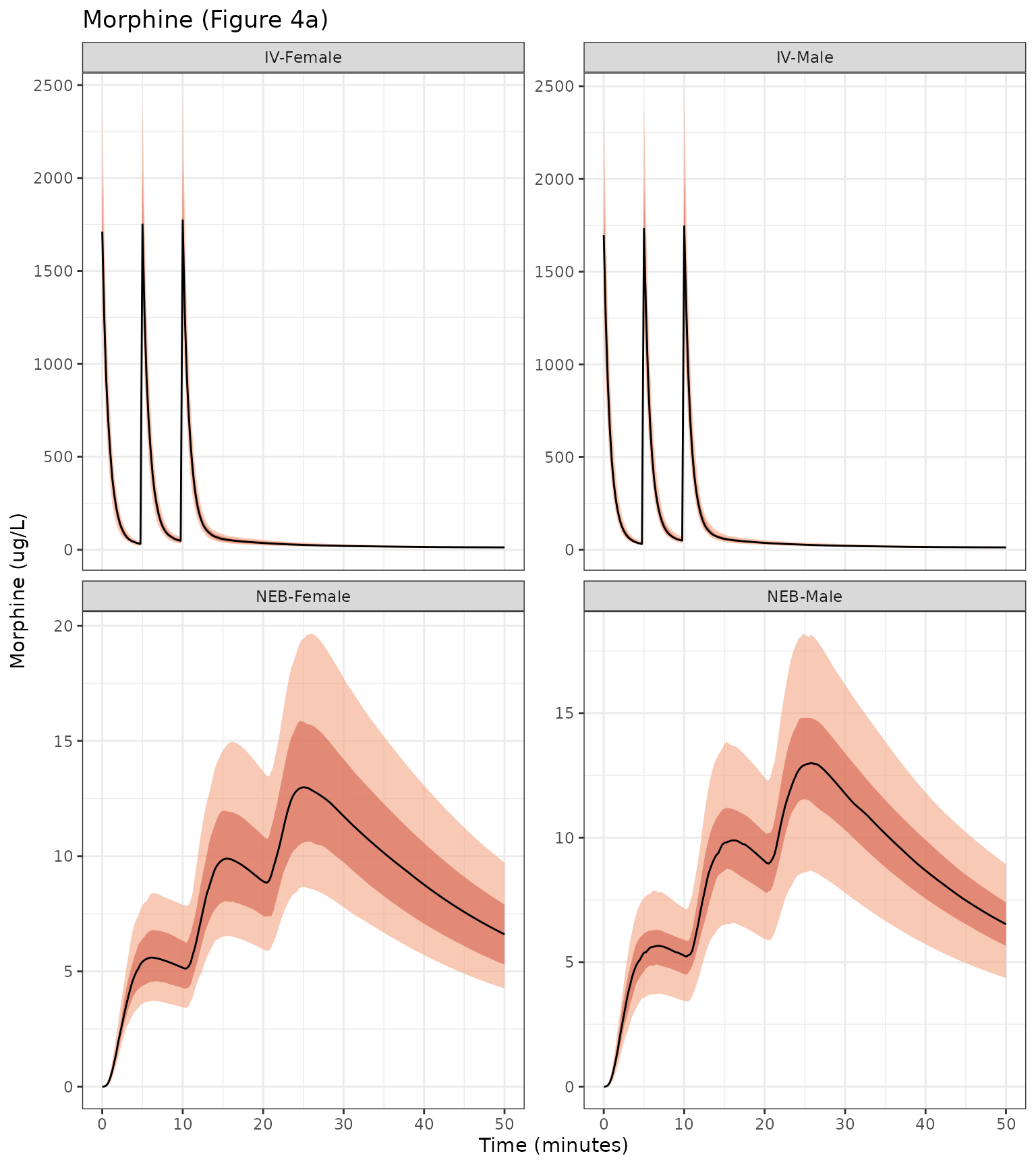
plot_fig4("M3G", 300) + ggtitle("M3G (Figure 4b)")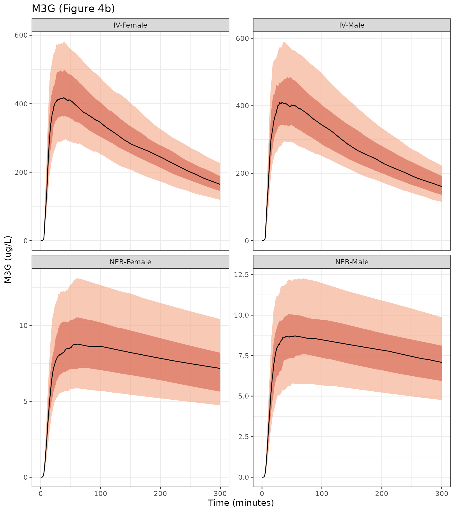
plot_fig4("M6G", 300) + ggtitle("M6G (Figure 4c)")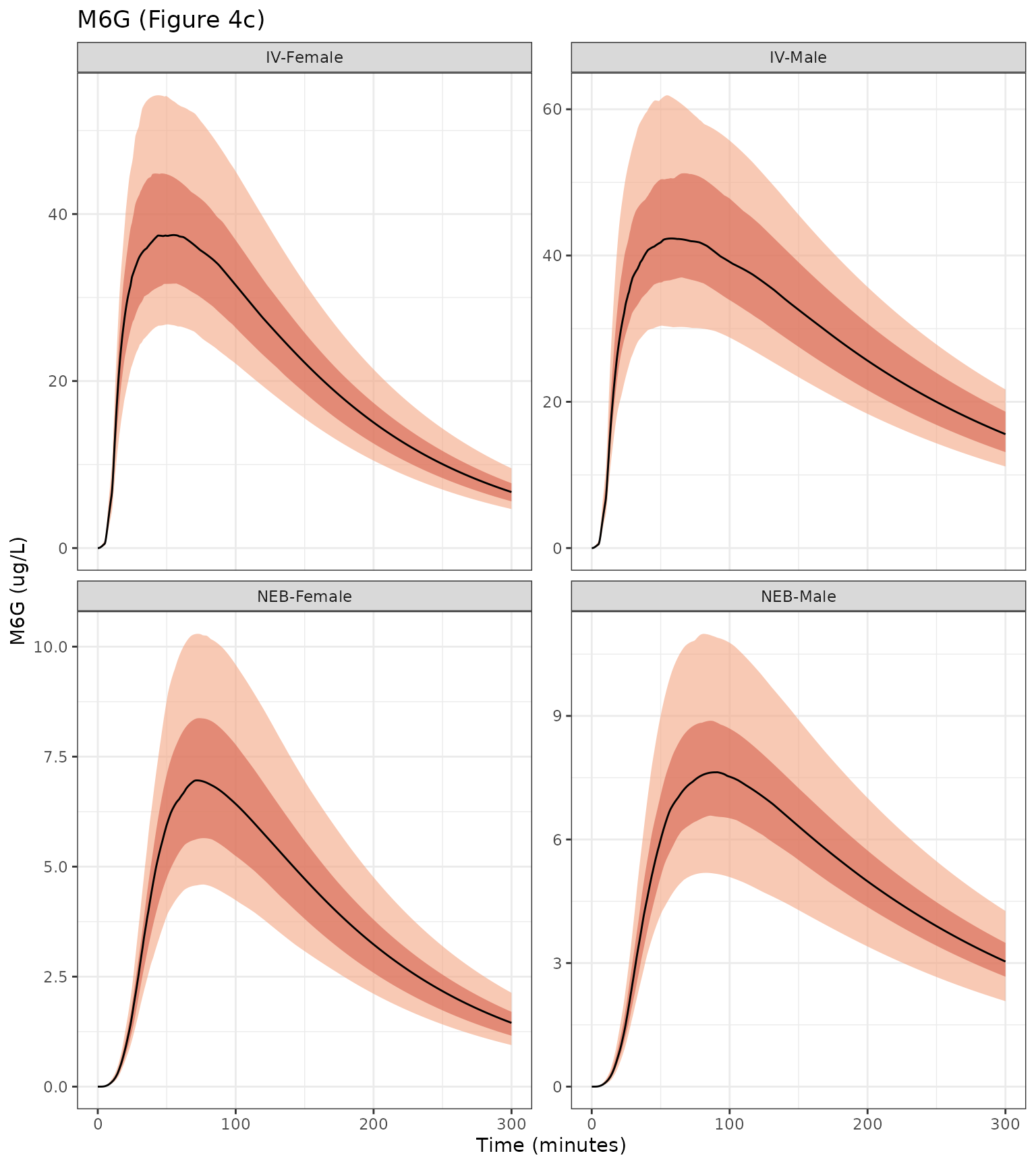
Replicates Figure 4 of Duflot 2022. The morphine panels reproduce the published figure directly: the i.v. peaks of about 1,750 ug/L and the nebulized medians of about 13 ug/L at 25 minutes and 6.5 ug/L at 50 minutes.
The glucuronide panels of Figure 4 are uniformly lower than this simulation by a factor of 285.34/461.46 = 0.618, the ratio of the morphine and glucuronide molecular weights. That is the pattern expected if the published glucuronide curves were converted from nmol/L to ug/L with the morphine molecular weight. The deposited dataset points the same way: its glucuronide concentrations, converted with 461.46 g/mol, reproduce the observed medians of Table 2 exactly. So the model output is converted with 461.46 g/mol throughout this vignette, and the table below compares against Figure 4 on both bases.
# Medians digitised by the maintainers from Figure 4 (median line; peak and
# the last plotted time, 50 min for nebulized morphine, 300 min otherwise).
fig4_digitised <- tibble::tribble(
  ~arm, ~analyte, ~metric, ~published,
  "NEB-Female", "Morphine", "peak", 12.8,
  "NEB-Female", "Morphine", "C50", 6.5,
  "NEB-Male", "Morphine", "peak", 12.6,
  "NEB-Male", "Morphine", "C50", 6.4,
  "IV-Female", "M3G", "peak", 255,
  "IV-Female", "M3G", "C300", 103,
  "IV-Male", "M3G", "peak", 262,
  "IV-Male", "M3G", "C300", 104,
  "NEB-Female", "M3G", "peak", 5.4,
  "NEB-Female", "M3G", "C300", 4.4,
  "NEB-Male", "M3G", "peak", 5.15,
  "NEB-Male", "M3G", "C300", 4.1,
  "IV-Female", "M6G", "peak", 25.7,
  "IV-Female", "M6G", "C300", 4.6,
  "IV-Male", "M6G", "peak", 27.3,
  "IV-Male", "M6G", "C300", 10.1,
  "NEB-Female", "M6G", "peak", 4.5,
  "NEB-Female", "M6G", "C300", 0.95,
  "NEB-Male", "M6G", "peak", 5.0,
  "NEB-Male", "M6G", "C300", 2.0
)

sim_metrics <- bands_fig4 |>
  dplyr::group_by(arm, analyte) |>
  dplyr::summarise(
    peak = max(median[time <= 300]),
    C50 = median[time == 50],
    C300 = median[time == 300],
    .groups = "drop"
  ) |>
  tidyr::pivot_longer(c(peak, C50, C300), names_to = "metric", values_to = "simulated")

fig4_cmp <- fig4_digitised |>
  dplyr::inner_join(sim_metrics, by = c("arm", "analyte", "metric")) |>
  dplyr::mutate(
    # Put the simulated glucuronides on the morphine-molecular-weight basis
    # that the published glucuronide curves appear to use.
    simulated_mw_basis = ifelse(analyte == "Morphine", simulated, simulated * mw_morphine / mw_glucuronide),
    pct_diff = 100 * (simulated_mw_basis - published) / published
  )

fig4_cmp |>
  dplyr::rename(
    "Arm" = arm, "Analyte" = analyte, "Metric" = metric,
    "Figure 4 (ug/L)" = published,
    "Simulated (ug/L)" = simulated,
    "Simulated, morphine-MW basis" = simulated_mw_basis,
    "% diff" = pct_diff
  ) |>
knitr::kable(digits = 2, caption = "Figure 4 medians vs. simulated medians.")| Arm | Analyte | Metric | Figure 4 (ug/L) | Simulated (ug/L) | Simulated, morphine-MW basis | % diff |
|---|---|---|---|---|---|---|
| NEB-Female | Morphine | peak | 12.80 | 12.99 | 12.99 | 1.47 |
| NEB-Female | Morphine | C50 | 6.50 | 6.61 | 6.61 | 1.66 |
| NEB-Male | Morphine | peak | 12.60 | 13.00 | 13.00 | 3.18 |
| NEB-Male | Morphine | C50 | 6.40 | 6.52 | 6.52 | 1.93 |
| IV-Female | M3G | peak | 255.00 | 417.47 | 258.14 | 1.23 |
| IV-Female | M3G | C300 | 103.00 | 164.28 | 101.58 | -1.38 |
| IV-Male | M3G | peak | 262.00 | 410.44 | 253.79 | -3.13 |
| IV-Male | M3G | C300 | 104.00 | 160.59 | 99.30 | -4.52 |
| NEB-Female | M3G | peak | 5.40 | 8.78 | 5.43 | 0.51 |
| NEB-Female | M3G | C300 | 4.40 | 7.17 | 4.43 | 0.75 |
| NEB-Male | M3G | peak | 5.15 | 8.72 | 5.39 | 4.67 |
| NEB-Male | M3G | C300 | 4.10 | 7.08 | 4.38 | 6.78 |
| IV-Female | M6G | peak | 25.70 | 37.49 | 23.18 | -9.81 |
| IV-Female | M6G | C300 | 4.60 | 6.71 | 4.15 | -9.86 |
| IV-Male | M6G | peak | 27.30 | 42.33 | 26.18 | -4.11 |
| IV-Male | M6G | C300 | 10.10 | 15.57 | 9.63 | -4.67 |
| NEB-Female | M6G | peak | 4.50 | 6.96 | 4.30 | -4.37 |
| NEB-Female | M6G | C300 | 0.95 | 1.45 | 0.90 | -5.66 |
| NEB-Male | M6G | peak | 5.00 | 7.63 | 4.72 | -5.61 |
| NEB-Male | M6G | C300 | 2.00 | 3.04 | 1.88 | -6.12 |
stopifnot(
  # Structural: a mis-transcribed rate constant, volume or covariate effect
  # moves these by tens of percent.
  abs(median(fig4_cmp$pct_diff)) < 10,
  # Envelope, robust to which checkpoints are noisiest to digitise.
  quantile(abs(fig4_cmp$pct_diff), 0.9) < 25
)
On the morphine-molecular-weight basis every checkpoint, including the sex difference in M6G elimination (about two-fold higher M6G in men at 300 minutes), agrees with Figure 4 to within digitisation error.
Assumptions and deviations
-
Glucuronide formation is anchored to model time
zero. Supplementary Material S4 writes the formation kernel as
exp(log(Ac) + log(ktr1) + N1*log(ktr1*t) - ktr1*t - LN1fac), i.e. the current morphine amount times a Savic gamma density evaluated at the model timet, not at the time after dose. The model transcribes this exactly. In the source data every participant received a single dose at time 0, and Figure 4 gives all doses within 20 minutes of the first, so the published use cases are reproduced. The M3G kernel is effectively zero after about 30 minutes and the M6G kernel after about 300 minutes; a dose given later than that on the same record forms little or no glucuronide. Start the record at the first dose, and do not use the model for regimens that extend much beyond the published 20-minute titration window. -
Morphine elimination. As in S4, morphine leaves the
central compartment only through the two glucuronidation outflows
(
ktr_m3g * centralandktr_m6g * central); the kernel scales how much of that outflow appears as glucuronide, so the model does not conserve mass between parent and metabolites. This is the published structure. - k13 route coefficient label. Table 3 prints the coefficient in the k13 row as ‘beta_km3_Route (=NEB)’. The covariate-building table (S3, ‘Route on k13’) and the Results text (k13 1.30 vs. 0.35 1/min for NEB vs. i.v.; 0.306 x exp(1.39) = 1.23) identify it as the route effect on k13.
- Direction of the M3G route effect. The Results text describes ‘a significantly higher M3G elimination (0.0038 vs. 0.0010)’ in the NEB context, but Table 3 gives km3 = 0.0038 1/min for the i.v. reference with beta = -1.33 for NEB (0.0010 1/min). The model follows Table 3; the Figure 4 replication (flat nebulized M3G profile) confirms this reading.
- Perfect correlation between k13 and km3. Table 3 reports corr_km3_k13 = -1, which makes the covariance block singular. The covariance was scaled by 0.99 (correlation -0.99) so the block can be sampled; both variances are kept exactly. The paper fixed omega_k13 (RSE ‘(-)’) while estimating omega_km3 and the correlation; nlmixr2 cannot fix one element of a block, so the block is left unfixed and the fixed status is recorded here and in the model comments.
-
Bioavailability transform. F was logit-normal in
Monolix but has no random effect and was fixed, so it is stored as
lfdepot = log(0.035). -
Route and sex coding. The paper codes route 0 =
i.v. / 1 = NEB and sex 0 = women / 1 = men. The model uses the canonical
ROUTE_IV(1 = i.v.) andSEXF(1 = female) columns and applies the paper’s coefficients to1 - ROUTE_IVand1 - SEXF, so every published value is carried unchanged. - Nebulization input. The 5-minute nebulization is a bolus into the transit depot, as in the authors’ dataset (no infusion duration); the transit chain describes the delay.
-
Undefined kernel before a nebulized dose. The
analytic absorption kernel depends on the time since the last
depotdose, which is undefined for an intravenous participant; the model holds the depot input at 0 until the first nebulized dose. - M3G below the observed data at the population level. The simulated median M3G concentrations are about 0.6 (NEB) to 0.75 (i.v.) of the observed medians of Table 2, and the simulated AUCs are about a third (i.v.) to a half (NEB) below Table 2’s model-derived AUCs, while morphine and M6G agree. The maintainers also compared typical-value predictions with the authors’ deposited dataset and saw the same ratio (observed M3G about 1.4-1.6 times the prediction), whereas the published Figure 4 matches this model exactly once its units are accounted for. The published population parameters therefore appear to under-predict M3G at the median. The individual fits (Figure 2) and the model-derived AUCs of Table 2 use individual parameters, which absorb it. No parameter was adjusted.
- Figure 4 glucuronide units. See the Figure 4 section: the published glucuronide curves are consistent with a conversion using the morphine molecular weight.
-
Covariates screened but not retained. Age, weight
and BMI were tested (mean-centred, log-transformed) and not retained;
they are recorded in
covariatesDataExcluded. - Errata. No correction notice for this article is linked in Europe PMC as of 2026-09-30.