Rifapentine (Francis 2019)
Source:vignettes/articles/Francis_2019_rifapentine.Rmd
Francis_2019_rifapentine.RmdModel and source
mod <- rxode2::rxode2(readModelDb("Francis_2019_rifapentine"))- Citation: Francis J, Zvada SP, Denti P, Hatherill M, Charalambous S, Mungofa S, Dawson R, Dorman S, Gupte N, Wiesner L, Jindani A, Harrison TS, Olagunju A, Egan D, Owen A, McIlleron HM. (2019). A population pharmacokinetic analysis shows that arylacetamide deacetylase (AADAC) gene polymorphism and HIV infection affect the exposure of rifapentine. Antimicrob Agents Chemother 63(4):e01964-18. doi:10.1128/AAC.01964-18.
- Description: One-compartment population pharmacokinetic model with first-order elimination and Savic transit-compartment absorption (NN = 10.2, MTT = 1.47 h) followed by a separate first-order absorption step (ka = 0.814 1/h) for oral rifapentine in 326 southern African adults with drug-susceptible pulmonary tuberculosis pooled from two trials (RIFAQUIN, 900 mg twice weekly or 1,200 mg once weekly in the continuation phase; Daily RPE, 450 or 600 mg daily in the intensive phase). Clearance is allometrically scaled on fat-free mass (reference 46 kg, exponent 0.75 fixed) and apparent volume on total body weight (reference 56 kg, exponent 1 fixed), giving typical values CL = 1.33 L/h and V = 25 L. Four covariate effects are carried: AADAC rs1803155 AA homozygotes have 10.4% lower clearance (the paper’s headline pharmacogenetic finding), the RIFAQUIN 1,200-mg-once-weekly arm has 13.2% lower clearance, HIV-positive patients have 21.9% lower bioavailability, and Daily RPE participants have 23.3% lower bioavailability than RIFAQUIN participants (attributed to non-standardised meals). Bioavailability is fixed to 1 in the RIFAQUIN HIV-negative reference. Inter-individual variability is on CL (23.0% CV) and V (12.8% CV); the paper’s inter-occasion variability on ka (48.9% CV), MTT (37.4% CV) and NN (20.3% CV) is carried as single-draw random effects because the source does not enumerate occasions - see the vignette Assumptions and deviations. Residual variability is combined additive (0.247 mg/L) plus proportional (9.56%).
- Article: doi:10.1128/AAC.01964-18
Rifapentine is a long-acting rifamycin used to treat drug-susceptible
tuberculosis. Its primary metabolic route is deacetylation to
25-desacetyl rifapentine by arylacetamide deacetylase (AADAC), which is
why that gene is the pharmacogenetic candidate of interest. Francis 2019
pooled two southern African trials to ask whether functionally
significant polymorphisms affecting OATP1B1, the pregnane X receptor,
the constitutive androstane receptor and AADAC change rifapentine
exposure. Five SNPs were genotyped and reported in Table 3 –
SLCO1B1 rs2306283 and rs4149032, NR1I2
rs2472677 and rs1523130, and AADAC rs1803155 – and only
AADAC rs1803155 was retained in the final model.
Population
The analysis pooled 1,144 rifapentine plasma concentrations from 326 patients with drug-susceptible pulmonary tuberculosis (1,151 measured; 7 below the 0.156 mg/L LLOQ were omitted). Patients came from two trials: the phase III RIFAQUIN study (ISRCTN44153044), whose continuation-phase arms gave 1,200 mg rifapentine once weekly (n = 125) or 900 mg twice weekly (n = 116) alongside moxifloxacin, and the Daily RPE study (NCT00814671), in which 450 mg (n = 44) or 600 mg (n = 41) rifapentine daily replaced rifampin during the intensive phase. Median age was 32 years (range 18-80), median weight 56 kg (38-94), median fat-free mass 45 kg (27-62); 108 of 326 (33.1%) were female and 59 of 326 (18.1%) were HIV-coinfected (Francis 2019 Table 1).
Pharmacogenetic data were available for 162 of the 326 patients
(49.7%), all from South African sites. The AADAC rs1803155
variant A allele was the major allele in this cohort at a frequency of
0.82, with 106 of 162 (65.4%) A/A, 53 (32.7%) G/A and only 3 (1.85%) G/G
(Francis 2019 Table 3). The source imputed the missing genotypes by
mixture modelling.
The two trials differed in how the dose was taken, and this turns out to matter more than the genotype: RIFAQUIN gave every dose with 240 ml of water 15 min after a standardised light meal of two hard-boiled eggs with bread, whereas Daily RPE advised patients to dose with food but neither standardised the meal nor recorded what was eaten.
The same information is available programmatically via
readModelDb("Francis_2019_rifapentine")()$population.
Source trace
Every ini() value carries an in-file comment naming its
source location. The table below collects them in one place for
review.
| Quantity | Value | Source location |
|---|---|---|
| CL/F (reference FFM 46 kg) | 1.33 L/h (95% CI 1.14, 1.54) | Table 2, row ‘CL (liters/h)’ |
| V/F (reference WT 56 kg) | 25 L (95% CI 21.9, 28.4) | Table 2, row ‘V (liters)’ |
| ka | 0.814 1/h (95% CI 0.568, 1.26) | Table 2, row ‘ka (h-1)’ |
| MTT | 1.47 h (95% CI 1.20, 1.78) | Table 2, row ‘MTT (h)’ |
| NN (transit-chain shape) | 10.2 (95% CI 6.70, 14.0) | Table 2, row ‘NN’ |
| F | 1 (fixed) | Table 2, row ‘F’ |
| Allometric exponent on CL (FFM) | 0.75 (fixed) | Methods, ‘as described by Anderson and Holford’ |
| Allometric exponent on V (WT) | 1 (fixed) | Methods, ‘as described by Anderson and Holford’ |
| AADAC rs1803155 AA on CL | -10.4% (95% CI -17.3, -3.53) | Table 2, row ‘AADAC rs1803155 (AA) effect on CL (%)’ |
| RIFAQUIN 1,200 mg arm on CL | -13.2% (95% CI -22.8, -4.36) | Table 2, row ‘Effect of group on 1,200-mg dose in RIFAQUIN study on CL (%)’ |
| HIV-positive on F | -21.9% (95% CI -33.2, -6.64) | Table 2, row ‘Effect of HIV + on F (%)’ |
| Daily RPE study on F | -23.3% (95% CI -35.6, -9.25) | Table 2, row ‘Effect of Daily RPE study on F (%)’ |
| IIV CL | 23.0% CV (95% CI 17.7, 28.6) | Table 2, ‘Variability’ column, CL row |
| IIV V | 12.8% CV (95% CI 8.8, 17.4) | Table 2, ‘Variability’ column, V row |
| IOV ka | 48.9% CV (95% CI 36.4, 59.8) | Table 2, ‘Variability’ column, ka row |
| IOV MTT | 37.4% CV (95% CI 28.3, 48.6) | Table 2, ‘Variability’ column, MTT row |
| IOV NN | 20.3% CV (95% CI 14.9, 26.4) | Table 2, ‘Variability’ column, NN row |
| Proportional residual error | 9.56% (95% CI 7.09, 13.2) | Table 2, row ‘Proportional residual error (%)’ |
| Additive residual error | 0.247 mg/L (95% CI 0.143, 0.401) | Table 2, row ‘Additive residual error (mg/liter)’ |
| Reference FFM / WT | 46 kg / 56 kg | Table 2, footnote b; Results paragraph 2 |
| Structural model | 1-compartment, first-order elimination, transit absorption | Results paragraph 2; Methods, ‘Pharmacokinetic analysis’ |
Random-effect variances are stored on the internal (log) scale as
omega^2 = log(1 + CV^2), the exact inverse of the
log-normal coefficient of variation, because Methods states “A lognormal
distribution was assumed for IIV and IOV”. See Assumptions and
deviations for the alternative reading.
Typical-value checks
All of the checks in this section are deterministic: random effects are zeroed and the covariates are set explicitly, so every assertion is an exact identity rather than a property of a random draw.
typ <- rxode2::zeroRe(mod)

## Solve one typical subject over `ncyc + 1` dosing intervals and summarise the
## final (steady-state) interval.
solve_typ <- function(dose, ii, ncyc, ffm = 46, wt = 56, hiv = 0, aadac = 0,
                      high = 0, daily = 0, dt = 0.05, model = typ) {
  ev <-
    rxode2::et(amt = dose, cmt = "depot", ii = ii, addl = ncyc) |>
    rxode2::et(seq(0, ii * (ncyc + 1), by = dt), cmt = "central") |>
    as.data.frame() |>
    dplyr::mutate(
      FFM = ffm, WT = wt, HIV_POS = hiv,
      SNP_AADAC_RS1803155_HOM = aadac, DOSE_HIGH = high,
      STUDY_DAILY_RPE = daily
    )
  rxode2::rxSolve(model, ev, omega = NA, returnType = "data.frame")
}

trapz <- function(x, y) sum(diff(x) * (utils::head(y, -1) + utils::tail(y, -1)) / 2)

summarise_tau <- function(s, dose, ii, ncyc) {
  last <- dplyr::filter(s, time >= ii * ncyc, time <= ii * (ncyc + 1))
  auctau <- trapz(last$time, last$Cc)
  tibble::tibble(
    cl = s$cl[1], vc = s$vc[1], fdepot = s$fdepot[1],
    half_life = log(2) * s$vc[1] / s$cl[1],
    auctau = auctau,
    mass_balance = s$cl[1] * auctau / (dose * s$fdepot[1]),
    cmax = max(last$Cc),
    tmax = last$time[which.max(last$Cc)] - ii * ncyc,
    ctrough = last$Cc[nrow(last)]
  )
}
Reference subject reproduces the published typical values
The reference patient of Table 2 footnote b has body weight 56 kg and
fat-free mass 46 kg, is HIV-negative, is not an AADAC
rs1803155 A/A homozygote, and is a RIFAQUIN participant outside the
1,200 mg arm. The model must return the Table 2 point estimates
exactly.
ref <- summarise_tau(solve_typ(900, 84, 20), 900, 84, 20)
knitr::kable(
  ref |>
    dplyr::transmute(
      `CL/F (L/h)` = cl, `V/F (L)` = vc, `F` = fdepot,
      `t1/2 (h)` = half_life, `AUCtau (mg*h/L)` = auctau,
      `Cmax (mg/L)` = cmax, `Tmax (h)` = tmax
    ),
  digits = 3
)| CL/F (L/h) | V/F (L) | F | t1/2 (h) | AUCtau (mg*h/L) | Cmax (mg/L) | Tmax (h) |
|---|---|---|---|---|---|---|
| 1.33 | 25 | 1 | 13.029 | 676.692 | 29.981 | 5.15 |
stopifnot(
  # Table 2 point estimates, recovered exactly at the reference covariates.
  isTRUE(all.equal(ref$cl, 1.33, tolerance = 1e-10)),
  isTRUE(all.equal(ref$vc, 25, tolerance = 1e-10)),
  isTRUE(all.equal(ref$fdepot, 1, tolerance = 1e-10))
)
The implied terminal half-life is 13 h, consistent with the “half-life of approximately 12 h in humans” quoted in the Introduction, and the typical Tmax is 5.2 h, consistent with “peak plasma concentrations being reached within 5 h”.
stopifnot(
  # Introduction: "Rifapentine has a half-life of approximately 12 h in humans".
  ref$half_life > 10, ref$half_life < 16,
  # Introduction: "peak plasma concentrations being reached within 5 h".
  ref$tmax > 3, ref$tmax < 6.5
)
Steady-state mass balance
At steady state the amount cleared over one dosing interval must
equal the amount absorbed, so CL * AUCtau == Dose * F
exactly. This is the one check the transit() /
f(depot) <- 0 absorption idiom cannot pass if the
gamma-density input silently evaluates to zero, and it also catches a
dose that arrives twice. A ratio of simulated-to-expected AUC would
not catch either failure, because it divides one wrong number
by another.
mb <- dplyr::bind_rows(
  summarise_tau(solve_typ(450, 24, 20, ffm = 47, wt = 55, daily = 1), 450, 24, 20),
  summarise_tau(solve_typ(600, 24, 20, ffm = 47, wt = 55, daily = 1), 600, 24, 20),
  summarise_tau(solve_typ(900, 84, 12, ffm = 45, wt = 55), 900, 84, 12),
  summarise_tau(solve_typ(1200, 168, 8, ffm = 45, wt = 57, high = 1), 1200, 168, 8)
) |>
  dplyr::mutate(Arm = c("DailyRPE-450", "DailyRPE-600", "RIFAQUIN-900", "RIFAQUIN-1200"), .before = 1)

knitr::kable(
  mb |>
    dplyr::transmute(
      Arm, `CL/F (L/h)` = cl, `F` = fdepot, `AUCtau (mg*h/L)` = auctau,
      `Cmax (mg/L)` = cmax, `Tmax (h)` = tmax, `Ctrough (mg/L)` = ctrough,
      `CL*AUCtau / (Dose*F)` = mass_balance
    ),
  digits = c(0, 3, 3, 1, 2, 2, 2, 8)
)| Arm | CL/F (L/h) | F | AUCtau (mg*h/L) | Cmax (mg/L) | Tmax (h) | Ctrough (mg/L) | CLAUCtau / (DoseF) |
|---|---|---|---|---|---|---|---|
| DailyRPE-450 | 1.352 | 0.767 | 255.4 | 16.05 | 4.70 | 5.95 | 1.000001 |
| DailyRPE-600 | 1.352 | 0.767 | 340.5 | 21.41 | 4.70 | 7.93 | 1.000000 |
| RIFAQUIN-900 | 1.308 | 1.000 | 687.9 | 30.52 | 5.15 | 0.49 | 1.000000 |
| RIFAQUIN-1200 | 1.136 | 1.000 | 1056.7 | 39.72 | 5.35 | 0.03 | 1.000000 |
The mass-balance gate is not vacuous
A gate that passes on a broken model is worse than no gate. Deliberately breaking the absorption input must make the check fail.
broken <- typ |> rxode2::model(d/dt(depot) <- -ka * depot)
broken_s <- solve_typ(900, 84, 12, ffm = 45, wt = 55, model = broken)
broken_mb <- summarise_tau(broken_s, 900, 84, 12)$mass_balance

stopifnot(
  # With the transit() input removed, nothing reaches the depot at all.
  max(broken_s$Cc) == 0,
  # ... so the mass-balance gate above must go to zero rather than stay at 1.
  broken_mb < 1e-8
)
Covariate effects reproduce the published percentages
cov_check <- tibble::tribble(
  ~Effect, ~simulated, ~published,
  "AADAC rs1803155 A/A on CL",
  solve_typ(900, 84, 4, aadac = 1)$cl[1] / 1.33 - 1, -0.104,
  "RIFAQUIN 1,200 mg arm on CL",
  solve_typ(900, 84, 4, high = 1)$cl[1] / 1.33 - 1, -0.132,
  "HIV-positive on F",
  solve_typ(900, 84, 4, hiv = 1)$fdepot[1] / 1 - 1, -0.219,
  "Daily RPE study on F",
  solve_typ(900, 84, 4, daily = 1)$fdepot[1] / 1 - 1, -0.233
)

knitr::kable(
  cov_check |>
    dplyr::transmute(
      Effect,
      `Simulated change (%)` = 100 * simulated,
      `Francis 2019 Table 2 (%)` = 100 * published
    ),
  digits = 3
)| Effect | Simulated change (%) | Francis 2019 Table 2 (%) |
|---|---|---|
| AADAC rs1803155 A/A on CL | -10.4 | -10.4 |
| RIFAQUIN 1,200 mg arm on CL | -13.2 | -13.2 |
| HIV-positive on F | -21.9 | -21.9 |
| Daily RPE study on F | -23.3 | -23.3 |
Allometric scaling must also reproduce the fixed Anderson-Holford exponents rather than some other power.
allo <- tibble::tibble(
  ffm_ratio = solve_typ(900, 84, 4, ffm = 92)$cl[1] / 1.33,
  wt_ratio = solve_typ(900, 84, 4, wt = 112)$vc[1] / 25
)
stopifnot(
  # Doubling FFM must scale CL by 2^0.75 and doubling WT must scale V by 2^1.
  isTRUE(all.equal(allo$ffm_ratio, 2^0.75, tolerance = 1e-10)),
  isTRUE(all.equal(allo$wt_ratio, 2, tolerance = 1e-10))
)
The transit chain is load bearing
AUCtau is Dose * F / CL whatever the
absorption model does, so an exposure-only check is blind to the transit
parameterisation. Quadrupling MTT on a single-dose solve must
move Tmax substantially; if the transit input were being discarded (for
example because rxode2 had silently switched to an analytic solution),
Tmax would not move.
single_dose_tmax <- function(model) {
  ev <-
    rxode2::et(amt = 900, cmt = "depot") |>
    rxode2::et(seq(0, 48, by = 0.05), cmt = "central") |>
    as.data.frame() |>
    dplyr::mutate(
      FFM = 46, WT = 56, HIV_POS = 0, SNP_AADAC_RS1803155_HOM = 0,
      DOSE_HIGH = 0, STUDY_DAILY_RPE = 0
    )
  s <- rxode2::rxSolve(model, ev, omega = NA, returnType = "data.frame")
  s$time[which.max(s$Cc)]
}

tmax_base <- single_dose_tmax(typ)
tmax_slow <- single_dose_tmax(rxode2::ini(typ, lmtt = log(4 * 1.47)))
#> ℹ change initial estimate of `lmtt` to `1.77155676191054`

stopifnot(
  # The ODE chain is integrated, not replaced by a closed-form solution.
  is.null(mod$linCmt),
  # Quadrupling MTT delays the peak by more than 2 h.
  tmax_slow - tmax_base > 2
)
c(tmax_base = tmax_base, tmax_slow = tmax_slow)
#> tmax_base tmax_slow
#>      5.15     10.70
Virtual cohort
Each of the four treatment arms is simulated at its published size (44, 41, 116 and 125 patients, 326 in total, matching Francis 2019 Table 1), so the cohort is the trial rather than an arbitrary sample. That is well inside the 200-per-arm cap this package applies to vignette simulations.
Weight is drawn log-normally at each arm’s Table 1 median; fat-free
mass is derived from weight using that arm’s median FFM-to-weight ratio
plus a small independent residual, because the two quantities are
strongly but not perfectly correlated and the paper reports only their
marginal distributions. HIV prevalence is set per arm from Table 1, and
the AADAC A/A frequency is the pooled 65.4% of Table 3.
rxode2::rxSetSeed(20190327)
set.seed(20190327)

arms <- tibble::tribble(
  ~arm,             ~n,  ~dose, ~ii,  ~ncyc, ~tfig, ~daily, ~high, ~hiv_pct, ~wt_med, ~ffm_med,
  "DailyRPE-450",   44L,   450,  24,    14L,    30,      1,     0,    0.136,      55,       47,
  "DailyRPE-600",   41L,   600,  24,    14L,    30,      1,     0,    0.171,      55,       47,
  "RIFAQUIN-900",  116L,   900,  84,     9L,    50,      0,     0,    0.259,      55,       45,
  "RIFAQUIN-1200", 125L,  1200, 168,     7L,    50,      0,     1,    0.128,      57,       45
)

make_covariates <- function(a) {
  wt <- exp(stats::rnorm(a$n, log(a$wt_med), 0.16))
  ffm <- wt * (a$ffm_med / a$wt_med) * exp(stats::rnorm(a$n, 0, 0.07))
  tibble::tibble(
    id = seq_len(a$n),
    WT = wt,
    FFM = ffm,
    HIV_POS = as.numeric(stats::runif(a$n) < a$hiv_pct),
    SNP_AADAC_RS1803155_HOM = as.numeric(stats::runif(a$n) < 0.654),
    DOSE_HIGH = a$high,
    STUDY_DAILY_RPE = a$daily
  )
}

simulate_arm <- function(a) {
  covs <- make_covariates(a)
  tstart <- a$ii * a$ncyc
  ## Dense grid through absorption (the 48.9% CV on ka needs it for an accurate
  ## trapezoidal AUC), coarser afterwards.
  grid <- sort(unique(c(seq(0, 12, by = 0.1), seq(12, a$ii, by = 0.5))))
  ev <-
    rxode2::et(amt = a$dose, cmt = "depot", ii = a$ii, addl = a$ncyc) |>
    rxode2::et(tstart + grid, cmt = "central") |>
    rxode2::et(id = seq_len(a$n)) |>
    as.data.frame() |>
    dplyr::left_join(covs, by = "id")
  rxode2::rxSolve(mod, ev, returnType = "data.frame", addDosing = FALSE) |>
    dplyr::mutate(arm = a$arm, dose = a$dose, tau = a$ii, tad = time - tstart)
}

sims <- dplyr::bind_rows(lapply(seq_len(nrow(arms)), function(i) simulate_arm(arms[i, ])))

## Guard against a silently-degenerate cohort.
stopifnot(
  nrow(sims) > 0,
  all(is.finite(sims$sim)),
  dplyr::n_distinct(sims$cl) == sum(arms$n),
  max(sims$Cc) > 0
)

knitr::kable(
  sims |>
    dplyr::distinct(arm, id, WT, FFM, HIV_POS, SNP_AADAC_RS1803155_HOM) |>
    dplyr::group_by(Arm = arm) |>
    dplyr::summarise(
      N = dplyr::n(),
      `Median WT (kg)` = stats::median(WT),
      `Median FFM (kg)` = stats::median(FFM),
      `HIV+ (%)` = 100 * mean(HIV_POS),
      `AADAC A/A (%)` = 100 * mean(SNP_AADAC_RS1803155_HOM),
      .groups = "drop"
    ),
  digits = 1
)| Arm | N | Median WT (kg) | Median FFM (kg) | HIV+ (%) | AADAC A/A (%) |
|---|---|---|---|---|---|
| DailyRPE-450 | 44 | 54.8 | 47.1 | 6.8 | 59.1 |
| DailyRPE-600 | 41 | 54.6 | 45.8 | 26.8 | 68.3 |
| RIFAQUIN-1200 | 125 | 55.5 | 43.5 | 12.0 | 68.8 |
| RIFAQUIN-900 | 116 | 54.9 | 44.3 | 27.6 | 60.3 |
Replicating Figure 1
Figure 1 of Francis 2019 is a visual predictive check on a log concentration scale, stratified by the four dose groups, with the 2.5th, 50th and 97.5th percentiles of the observations drawn as red lines and the 95% confidence intervals of the same percentiles from the model’s own re-simulations drawn as shaded bands. The panel below reproduces it from this implementation.
pct <- sims |>
  dplyr::group_by(arm, tad) |>
  dplyr::summarise(
    lo = stats::quantile(sim, 0.025),
    mid = stats::median(sim),
    hi = stats::quantile(sim, 0.975),
    .groups = "drop"
  ) |>
  dplyr::left_join(dplyr::select(arms, arm, tfig), by = "arm") |>
  dplyr::filter(tad <= tfig)

ggplot2::ggplot(pct, ggplot2::aes(x = tad)) +
  ggplot2::geom_ribbon(ggplot2::aes(ymin = lo, ymax = hi), fill = "steelblue", alpha = 0.25) +
  ggplot2::geom_line(ggplot2::aes(y = mid), colour = "firebrick", linewidth = 0.8) +
  ggplot2::geom_line(ggplot2::aes(y = lo), colour = "firebrick", linetype = "dashed") +
  ggplot2::geom_line(ggplot2::aes(y = hi), colour = "firebrick", linetype = "dashed") +
  ggplot2::scale_y_log10() +
  ggplot2::facet_wrap(~arm, nrow = 1, scales = "free_x") +
  ggplot2::labs(
    x = "Time after dose (h)", y = "Rifapentine (mg/L)",
    title = "Replicates Figure 1 of Francis 2019"
  ) +
  ggplot2::theme_bw()
#> Warning in transformation$transform(x): NaNs produced
#> Warning in ggplot2::scale_y_log10(): log-10 transformation introduced infinite
#> values.
#> Warning in transformation$transform(x): NaNs produced
#> Warning in ggplot2::scale_y_log10(): log-10 transformation introduced infinite
#> values.
#> Warning: Removed 25 rows containing missing values or values outside the scale range
#> (`geom_ribbon()`).
#> Warning: Removed 25 rows containing missing values or values outside the scale range
#> (`geom_line()`).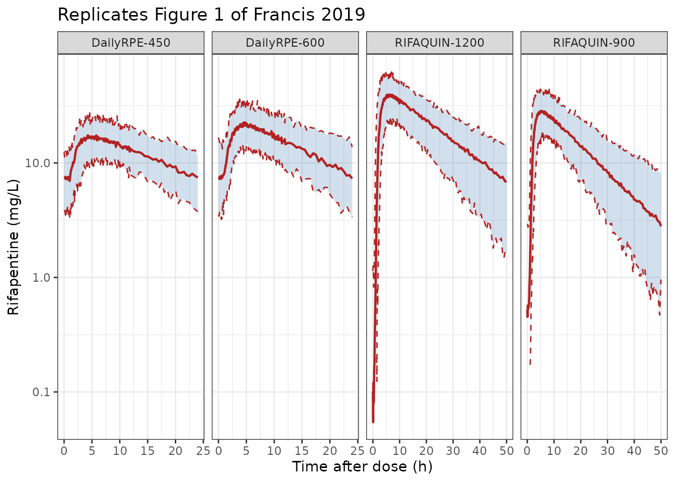
Quantitative comparison against Figure 1
Francis 2019 reports no numeric NCA table, so Figure 1 is the only published per-arm exposure summary available to check against. The most informative target in it is not the observed median line but the shaded band around it, which is the 95% confidence interval of the model-predicted median. Comparing this implementation’s median against that band is a model-versus-model check: it asks whether the re-implementation reproduces the published fit, without inheriting the binning and sampling noise of the observed line.
The band edges below were digitised from Figure 1 by locating the band’s characteristic fill colour column by column and converting pixel rows through the log axis calibrated on its 1 / 10 / 100 gridlines. Bins spanning the steep absorption limb are excluded, because there the flat per-bin band cannot be compared against a curve that moves several-fold across the same bin.
bands <- tibble::tribble(
  ~arm,             ~tad, ~lower, ~upper,
  "DailyRPE-450",     14,   9.03,  13.03,
  "DailyRPE-450",     22,   5.86,   9.41,
  "DailyRPE-600",     14,  12.51,  17.91,
  "DailyRPE-600",     22,   7.99,  13.46,
  "RIFAQUIN-900",     14,  18.81,  24.81,
  "RIFAQUIN-900",     36,   6.16,   8.12,
  "RIFAQUIN-900",     48,   3.31,   4.74,
  "RIFAQUIN-1200",    14,  22.14,  33.28,
  "RIFAQUIN-1200",    36,  10.21,  12.72,
  "RIFAQUIN-1200",    52,   6.06,   7.99
)

band_cmp <- bands |>
  dplyr::rowwise() |>
  dplyr::mutate(
    simulated = stats::median(sims$sim[sims$arm == arm & abs(sims$tad - tad) < 0.26])
  ) |>
  dplyr::ungroup() |>
  dplyr::mutate(
    inside = simulated >= lower & simulated <= upper,
    ## Distance outside the band, as a fraction of the band's own midpoint.
    excess = pmax(0, lower - simulated, simulated - upper) / ((lower + upper) / 2)
  )

knitr::kable(
  band_cmp |>
    dplyr::transmute(
      Arm = arm, `Time after dose (h)` = tad,
      `Figure 1 band, lower (mg/L)` = lower,
      `Figure 1 band, upper (mg/L)` = upper,
      `Simulated median (mg/L)` = simulated,
      `Inside band` = inside
    ),
  digits = 2
)| Arm | Time after dose (h) | Figure 1 band, lower (mg/L) | Figure 1 band, upper (mg/L) | Simulated median (mg/L) | Inside band |
|---|---|---|---|---|---|
| DailyRPE-450 | 14 | 9.03 | 13.03 | 12.06 | TRUE |
| DailyRPE-450 | 22 | 5.86 | 9.41 | 7.81 | TRUE |
| DailyRPE-600 | 14 | 12.51 | 17.91 | 13.62 | TRUE |
| DailyRPE-600 | 22 | 7.99 | 13.46 | 9.03 | TRUE |
| RIFAQUIN-900 | 14 | 18.81 | 24.81 | 19.07 | TRUE |
| RIFAQUIN-900 | 36 | 6.16 | 8.12 | 6.06 | FALSE |
| RIFAQUIN-900 | 48 | 3.31 | 4.74 | 3.48 | TRUE |
| RIFAQUIN-1200 | 14 | 22.14 | 33.28 | 28.80 | TRUE |
| RIFAQUIN-1200 | 36 | 10.21 | 12.72 | 11.94 | TRUE |
| RIFAQUIN-1200 | 52 | 6.06 | 7.99 | 6.67 | TRUE |
stopifnot(
  # Every comparison point has a simulated value (no vacuously-empty filter).
  nrow(band_cmp) == 10L, all(is.finite(band_cmp$simulated)),
  # The centre of the comparison: most points land inside the published band.
  sum(band_cmp$inside) >= 7L,
  # And no point strays far outside it. A mis-transcribed dose, clearance,
  # volume or bioavailability would move a whole arm by tens of percent.
  max(band_cmp$excess) < 0.15
)
For completeness the observed median line of Figure 1 was digitised the same way, over its descending limb where the three red lines are unambiguously ordered. This is a softer target – it is a binned median of the real data, so it carries the sampling noise of 41 to 125 patients and the paper’s own binning choices – so it is checked on the centre and on a robust quantile rather than point by point.
observed <- tibble::tribble(
  ~arm,             ~tad, ~median_obs,
  "DailyRPE-450",   10.8,       15.15,
  "DailyRPE-450",   16.4,       12.11,
  "DailyRPE-450",   20.1,       10.12,
  "DailyRPE-600",   11.9,       18.43,
  "DailyRPE-600",   16.0,       16.44,
  "DailyRPE-600",   23.5,       13.16,
  "RIFAQUIN-900",   11.7,       26.38,
  "RIFAQUIN-900",   20.0,       16.37,
  "RIFAQUIN-900",   24.0,       12.98,
  "RIFAQUIN-900",   30.0,        9.88,
  "RIFAQUIN-900",   48.0,        4.44,
  "RIFAQUIN-1200",  11.8,       34.66,
  "RIFAQUIN-1200",  20.0,       23.25,
  "RIFAQUIN-1200",  24.4,       18.81,
  "RIFAQUIN-1200",  30.0,       14.85,
  "RIFAQUIN-1200",  48.0,        6.96
)

obs_cmp <- observed |>
  dplyr::rowwise() |>
  dplyr::mutate(
    median_sim = stats::median(sims$sim[sims$arm == arm & abs(sims$tad - tad) < 0.26])
  ) |>
  dplyr::ungroup() |>
  dplyr::mutate(pct_diff = 100 * (median_sim - median_obs) / median_obs)

knitr::kable(
  obs_cmp |>
    dplyr::transmute(
      Arm = arm, `Time after dose (h)` = tad,
      `Figure 1 observed median (mg/L)` = median_obs,
      `Simulated median (mg/L)` = median_sim,
      `Difference (%)` = pct_diff
    ),
  digits = 2
)| Arm | Time after dose (h) | Figure 1 observed median (mg/L) | Simulated median (mg/L) | Difference (%) |
|---|---|---|---|---|
| DailyRPE-450 | 10.8 | 15.15 | 13.78 | -9.06 |
| DailyRPE-450 | 16.4 | 12.11 | 10.84 | -10.51 |
| DailyRPE-450 | 20.1 | 10.12 | 9.31 | -7.98 |
| DailyRPE-600 | 11.9 | 18.43 | 15.68 | -14.92 |
| DailyRPE-600 | 16.0 | 16.44 | 11.86 | -27.84 |
| DailyRPE-600 | 23.5 | 13.16 | 7.84 | -40.42 |
| RIFAQUIN-900 | 11.7 | 26.38 | 21.53 | -18.40 |
| RIFAQUIN-900 | 20.0 | 16.37 | 13.81 | -15.61 |
| RIFAQUIN-900 | 24.0 | 12.98 | 11.45 | -11.79 |
| RIFAQUIN-900 | 30.0 | 9.88 | 8.23 | -16.71 |
| RIFAQUIN-900 | 48.0 | 4.44 | 3.48 | -21.67 |
| RIFAQUIN-1200 | 11.8 | 34.66 | 33.14 | -4.38 |
| RIFAQUIN-1200 | 20.0 | 23.25 | 23.12 | -0.55 |
| RIFAQUIN-1200 | 24.4 | 18.81 | 20.04 | 6.54 |
| RIFAQUIN-1200 | 30.0 | 14.85 | 15.58 | 4.92 |
| RIFAQUIN-1200 | 48.0 | 6.96 | 7.45 | 6.97 |
stopifnot(
  nrow(obs_cmp) == 16L, all(is.finite(obs_cmp$median_sim)),
  # Centre: a mis-transcribed structural value moves the whole distribution
  # by tens of percent, well past the binning bias discussed below.
  abs(stats::median(obs_cmp$pct_diff)) < 25,
  # Envelope, robust to which bins the digitisation reads least well.
  stats::quantile(abs(obs_cmp$pct_diff), 0.9) < 40
)
The simulated medians sit 11.2% below the digitised observed medians on average. A residual bias of this size is expected rather than alarming: the published line is a binned median plotted at a representative time within a wide bin (the orange rug at the foot of Figure 1 marks bin edges at roughly 0.7, 4.5, 10, 17.5 and 30 h for the Daily RPE panels), whereas the simulated value is read at a single instant. The model-versus-model band comparison above is free of that artefact, and there the agreement is close.
PKNCA validation
The non-compartmental analysis below runs on ipredSim,
the individual predictions, rather than on sim. Residual
error is deliberately excluded here because this section’s purpose is to
check the model’s exposures against closed forms; leaving it in
would blunt the identity CL * AUC0-tau == Dose * F into a
noise tolerance and hide a real structural error behind it. The Figure 1
comparison above does the opposite and uses sim, because
the published percentiles are percentiles of observations and therefore
carry residual error.
conc_data <- sims |>
  dplyr::filter(!is.na(ipredSim)) |>
  dplyr::transmute(
    id = paste(arm, id, sep = "-"),
    treatment = arm,
    time = tad,
    conc = ipredSim
  )

dose_data <- sims |>
  dplyr::distinct(arm, id, dose, tau) |>
  dplyr::transmute(
    id = paste(arm, id, sep = "-"),
    treatment = arm,
    time = 0,
    amt = dose,
    tau = tau
  )

conc_obj <- PKNCA::PKNCAconc(
  conc_data, conc ~ time | treatment + id,
  concu = "mg/L", timeu = "h"
)
dose_obj <- PKNCA::PKNCAdose(
  dose_data, amt ~ time | treatment + id,
  doseu = "mg"
)

intervals <- dose_data |>
  dplyr::distinct(treatment, tau) |>
  dplyr::transmute(
    treatment,
    start = 0, end = tau,
    cmax = TRUE, tmax = TRUE, auclast = TRUE, half.life = TRUE, cmin = TRUE
  )

nca <- PKNCA::pk.nca(PKNCA::PKNCAdata(conc_obj, dose_obj, intervals = intervals))

nca_summary <- as.data.frame(nca) |>
  dplyr::filter(PPTESTCD %in% c("cmax", "tmax", "auclast", "half.life", "cmin")) |>
  dplyr::group_by(treatment, PPTESTCD) |>
  dplyr::summarise(median = stats::median(PPORRES), .groups = "drop") |>
  tidyr::pivot_wider(names_from = PPTESTCD, values_from = median)

knitr::kable(
  nca_summary |>
    dplyr::rename(
      "Arm" = treatment,
      "AUC0-tau (mg*h/L)" = auclast,
      "Cmax (mg/L)" = cmax,
      "Cmin (mg/L)" = cmin,
      "t1/2 (h)" = half.life,
      "Tmax (h)" = tmax
    ),
  digits = 2
)| Arm | AUC0-tau (mg*h/L) | Cmax (mg/L) | Cmin (mg/L) | t1/2 (h) | Tmax (h) |
|---|---|---|---|---|---|
| DailyRPE-450 | 292.55 | 17.36 | 7.25 | 15.11 | 4.75 |
| DailyRPE-600 | 327.50 | 22.08 | 7.21 | 12.95 | 4.50 |
| RIFAQUIN-1200 | 1188.60 | 40.77 | 0.06 | 16.91 | 5.70 |
| RIFAQUIN-900 | 661.60 | 28.90 | 0.50 | 13.36 | 5.20 |
Per-subject NCA reproduces the closed form
At steady state each subject’s own CL * AUC0-tau must
equal that subject’s Dose * F. Running the identity through
PKNCA rather than through the trapezoidal sum computed above tests the
NCA path as well as the model.
per_subject <- sims |>
  dplyr::distinct(arm, id, cl, fdepot, dose) |>
  dplyr::mutate(id = paste(arm, id, sep = "-"))

auc_check <- as.data.frame(nca) |>
  dplyr::filter(PPTESTCD == "auclast") |>
  dplyr::transmute(id, auctau = PPORRES) |>
  dplyr::inner_join(per_subject, by = "id") |>
  dplyr::mutate(recovery = cl * auctau / (dose * fdepot))

knitr::kable(
  auc_check |>
    dplyr::group_by(Arm = arm) |>
    dplyr::summarise(
      N = dplyr::n(),
      `Median CL*AUCtau / (Dose*F)` = stats::median(recovery),
      `Min` = min(recovery),
      `Max` = max(recovery),
      .groups = "drop"
    ),
  digits = 4
)| Arm | N | Median CLAUCtau / (DoseF) | Min | Max |
|---|---|---|---|---|
| DailyRPE-450 | 44 | 1 | 1 | 1 |
| DailyRPE-600 | 41 | 1 | 1 | 1 |
| RIFAQUIN-1200 | 125 | 1 | 1 | 1 |
| RIFAQUIN-900 | 116 | 1 | 1 | 1 |
NCA half-life recovers the model’s own disposition
hl_check <- as.data.frame(nca) |>
  dplyr::filter(PPTESTCD == "half.life") |>
  dplyr::transmute(id, hl_nca = PPORRES) |>
  dplyr::inner_join(
    sims |>
      dplyr::distinct(arm, id, cl, vc) |>
      dplyr::mutate(id = paste(arm, id, sep = "-"), hl_model = log(2) * vc / cl),
    by = "id"
  ) |>
  dplyr::mutate(pct_diff = 100 * (hl_nca - hl_model) / hl_model)

knitr::kable(
  hl_check |>
    dplyr::group_by(Arm = arm) |>
    dplyr::summarise(
      `Median NCA t1/2 (h)` = stats::median(hl_nca),
      `Median model t1/2 (h)` = stats::median(hl_model),
      `Median difference (%)` = stats::median(pct_diff),
      .groups = "drop"
    ),
  digits = 2
)| Arm | Median NCA t1/2 (h) | Median model t1/2 (h) | Median difference (%) |
|---|---|---|---|
| DailyRPE-450 | 15.11 | 14.95 | 0.81 |
| DailyRPE-600 | 12.95 | 12.81 | 0.69 |
| RIFAQUIN-1200 | 16.91 | 16.87 | 0.11 |
| RIFAQUIN-900 | 13.36 | 13.28 | 0.32 |
stopifnot(
  # Noise-free individual predictions, so the only slack is lambda-z window
  # selection on a finite grid.
  abs(stats::median(hl_check$pct_diff)) < 3,
  stats::quantile(abs(hl_check$pct_diff), 0.9) < 5
)
The AADAC A/A effect the paper was written to report is
a 10.4% clearance reduction. Against 23.0% CV inter-individual
variability on clearance it is, as the authors themselves conclude,
“modest and unlikely to be of clinical relevance”; the exposure
separation it produces in the simulated cohort is shown below for
context.
aadac_exposure <- auc_check |>
  dplyr::inner_join(
    sims |>
      dplyr::distinct(arm, id, SNP_AADAC_RS1803155_HOM) |>
      dplyr::mutate(id = paste(arm, id, sep = "-")),
    by = c("id", "arm")
  ) |>
  dplyr::group_by(Arm = arm, `AADAC A/A` = SNP_AADAC_RS1803155_HOM == 1) |>
  dplyr::summarise(N = dplyr::n(), `Median AUCtau (mg*h/L)` = stats::median(auctau), .groups = "drop")

knitr::kable(aadac_exposure, digits = 1)| Arm | AADAC A/A | N | Median AUCtau (mg*h/L) |
|---|---|---|---|
| DailyRPE-450 | FALSE | 18 | 255.2 |
| DailyRPE-450 | TRUE | 26 | 314.8 |
| DailyRPE-600 | FALSE | 13 | 297.7 |
| DailyRPE-600 | TRUE | 28 | 360.7 |
| RIFAQUIN-1200 | FALSE | 39 | 1101.4 |
| RIFAQUIN-1200 | TRUE | 86 | 1222.7 |
| RIFAQUIN-900 | FALSE | 46 | 589.0 |
| RIFAQUIN-900 | TRUE | 70 | 718.8 |
Assumptions and deviations
-
Reference fat-free mass is 46 kg, not 45 kg.
Francis 2019 reports the reference size twice in the body of the paper
as “body weight of 56 kg and FFM of 46 kg” (Table 2 footnote b) and “In
a typical patient (FFM, 46 kg; weight, 56 kg)” (Results), but the
Abstract instead says “body weight, 56 kg; fat-free mass, 45 kg”, which
is also the Table 1 pooled cohort median. The 46 kg reading is used here
because it sits in the parameter table’s own footnote and is repeated in
the Results body. The choice changes typical clearance by
(46/45)^0.75, that is 1.7%, so no conclusion in this vignette turns on it. -
Inter-occasion variability is carried as single-draw random
effects. Table 2 labels the variability on ka, MTT and NN as
IOV rather than IIV, but the paper never states how many pharmacokinetic
occasions a patient contributed, and both trials describe a single
sampling visit (RIFAQUIN during treatment month 4, Daily RPE at about
month 1). The published variances are therefore carried on
etalka,etalmttandetalnnas ordinary subject-level random effects, which reproduces the published magnitudes exactly for the one-occasion simulations used here. A user simulating more than one occasion per subject must redraw those three etas per occasion while holdingetalclandetalvcfixed. No occasion count was invented. -
Random-effect scale. Table 2 reports variability as
“% CV” and Methods states that a log-normal distribution was assumed, so
variances are stored as
omega^2 = log(1 + CV^2). The paper does not print the formula it used to convert its NONMEMOMEGAestimates into the CV column. The common alternative convention,omega^2 = CV^2, would make the largest variance (ka, 48.9% CV) 0.239 instead of 0.214, that is an 11% difference in variance or 5% in standard deviation. The same convention is used by the sibling rifapentine modelZvada_2010_rifapentinefrom the same research group. -
Transit-chain convention. The model uses the Savic
parameterisation
ktr = (NN + 1) / MTT, which is what rxode2’stransit()implements, with a separately estimatedkaon the final step out of the depot. Francis 2019 cites Savic et al. as its transit-model reference and reports the same three quantities (ka,MTT,NN) at nearly the same values asZvada_2010_rifapentine(NN 10.9, MTT 1.45 h), which is the same group’s earlier rifapentine model and uses this convention. No control stream is available to confirm it directly. The alternativektr = NN / MTTreading found in some other groups’ work would shorten the transit chain by one transfer; it would leave every AUC in this vignette untouched, which is why the Tmax sensitivity check above is included as a separate structural gate. - Dosing intervals for the RIFAQUIN arms. The paper describes 900 mg “twice weekly” and 1,200 mg “once weekly” without giving the day-of-week pattern. The simulations use a uniform 84 h interval for the twice-weekly arm and 168 h for the once-weekly arm. Because the terminal half-life is about 13 h, 84 h is more than six half-lives and accumulation is negligible, so an alternating 72 h / 96 h pattern would give effectively identical exposures.
-
Covariate distributions in the virtual cohort.
Francis 2019 Table 1 reports per-arm medians and ranges for weight and
fat-free mass but not their joint distribution, so weight is drawn
log-normally at the arm median and fat-free mass is derived from it
using the arm’s median FFM-to-weight ratio with a small independent
residual. HIV prevalence is the per-arm Table 1 percentage and the
AADACA/A frequency is the pooled 65.4% of Table 3 applied to every arm; the paper reports genotype frequencies only for the pooled genotyped subset. - Figure 1 values are digitised. The Figure 1 comparison targets were read off the published image, not from a table, because the paper reports no numeric exposure summary. They carry the error of that process, which is why the observed-median comparison is asserted on its centre and a robust quantile rather than point by point, and why the band comparison allows a small excursion outside each band.
-
Sex, age and the four non-retained SNPs are not in the
model. Francis 2019 screened
SLCO1B1rs2306283 and rs4149032,NR1I2rs2472677 and rs1523130 in addition toAADACrs1803155, and none of the four was retained; the Discussion notes that allometric scaling on fat-free mass already absorbed the variability otherwise attributable to sex. Those covariates therefore have no coefficient to transcribe and do not appear incovariateData. -
The 1,200 mg clearance effect is confounded with dosing
frequency. The
DOSE_HIGHindicator marks the RIFAQUIN 1,200-mg-once-weekly arm, which is the only once-weekly arm in the pool. The Discussion attributes the 13.2% lower clearance to reduced autoinduction under less frequent dosing rather than to the dose level, and explicitly contrasts the finding with an earlier report of decreased bioavailability at higher rifapentine doses. It must not be reused as a concentration-dependent saturation term. -
The Daily RPE study indicator is a proxy for food.
The 23.3% bioavailability reduction is attributed by the authors to
non-standardised meals in Daily RPE against a standardised light meal in
RIFAQUIN, not to anything intrinsic to the trial. A user simulating a
standardised fed dose should set
STUDY_DAILY_RPE = 0whichever trial the remaining covariates come from. ```