GS-441524 after remdesivir (Sukeishi 2022)
Source:vignettes/articles/Sukeishi_2022_remdesivir.Rmd
Sukeishi_2022_remdesivir.RmdModel and source
ui <- rxode2::rxode(readModelDb("Sukeishi_2022_remdesivir"))
#> ℹ parameter labels from comments will be replaced by 'label()'- Citation: Sukeishi A, Itohara K, Yonezawa A, Sato Y, Matsumura K, Katada Y, Nakagawa T, Hamada S, Tanabe N, Imoto E, Kai S, Hirai T, Yanagita M, Ohtsuru S, Terada T, Ito I. Population pharmacokinetic modeling of GS-441524, the active metabolite of remdesivir, in Japanese COVID-19 patients with renal dysfunction. CPT Pharmacometrics Syst Pharmacol. 2022;11(1):94-103. doi:10.1002/psp4.12736
- Article: https://doi.org/10.1002/psp4.12736 (open access, PMC8646568)
- Supporting Information: Tables S1-S2 (stepwise covariate search) and the NONMEM control stream of the final model.
ui
#>  ── rxode2-based free-form 1-cmt ODE model ──────────────────────────────────────
#>  ── Initalization: ──
#> Fixed Effects ($theta):
#>            lcl            lvc      e_crcl_cl e_age_ge_75_vc         propSd
#>       2.468100       5.945421       1.090000      -0.429000       0.152000
#>
#> Omega ($omega):
#>          etalcl   etalvc
#> etalcl 0.065431 0.000000
#> etalvc 0.000000 0.112457
#> attr(,"lotriLabels")
#> [1] "Sukeishi 2022 Table 2: IIV for CL = 26.0 CV% (RSE 9.6%, shrinkage 4.22%) -> log(0.260^2 + 1)"
#> [2] "Sukeishi 2022 Table 2: IIV for Vd = 34.5 CV% (RSE 12.8%, shrinkage 24.1%) -> log(0.345^2 + 1)"
#> attr(,"lotriFix")
#>        etalcl etalvc
#> etalcl  FALSE  FALSE
#> etalvc  FALSE  FALSE
#>
#> States ($state or $stateDf):
#>   Compartment Number Compartment Name
#> 1                  1          central
#>  ── μ-referencing ($muRefTable): ──
#>   theta    eta level covariates
#> 1   lcl etalcl    id
#> 2   lvc etalvc    id
#>
#>  ── Model (Normalized Syntax): ──
#> function() {
#>     compartmentData <- list(central = list(analyte = "GS-441524",
#>         units = "mg", specimen = "serum", verified = TRUE))
#>     covariateData <- list(CRCL = list(description = "Estimated glomerular filtration rate, BSA-normalized (eGFR indexed), from the Japanese-coefficient MDRD equation on standardized serum creatinine.",
#>         units = "mL/min/1.73 m^2", type = "continuous", reference_category = NULL,
#>         notes = "Sukeishi 2022 Methods 'Patients and data collection': the clinical laboratory reported eGFR indexed (mL/min/1.73 m^2) from the Modification of Diet in Renal Disease equation for Japanese, and the authors de-indexed it to absolute mL/min as eGFR non-indexed = eGFR indexed / 1.73 * BSA, with BSA from the Du Bois equation. The final model uses the ABSOLUTE value (Table 2: CL = theta_CL * (eGFR non-indexed / 74.7)^theta), which gave a better fit than eGFR indexed, creatinine clearance or serum creatinine (Results 'PopPK model and model evaluation'). This file therefore takes the canonical BSA-normalized CRCL plus BSA and performs the same de-indexing inside model(); supply CRCL on the mL/min/1.73 m^2 scale, not absolute mL/min, or the renal term is rescaled by BSA/1.73. Time-varying in the source: the covariate was the value at each concentration measurement point. Observed eGFR non-indexed range 16.4-147.7 mL/min (median 74.7). In the Supporting Information control stream the absolute value is the data column EGFR2 (CL = THETA(1)*(EGFR2/74.7)**THETA(3)*EXP(ETA(1))).",
#>         source_name = "eGFRindexed"), BSA = list(description = "Body surface area (Du Bois equation)",
#>         units = "m^2", type = "continuous", reference_category = NULL,
#>         notes = "Used only to de-index eGFR (eGFR non-indexed = CRCL / 1.73 * BSA), per Sukeishi 2022 Methods 'Patients and data collection'. BSA was also screened directly on CL and V but not retained. Cohort median 1.8 m^2 (range 1.24-2.21), Table 1.",
#>         source_name = "BSA"), AGE = list(description = "Age",
#>         units = "years", type = "continuous", reference_category = NULL,
#>         notes = "Enters only through the binary indicator AGE >= 75 years on the volume of distribution (Sukeishi 2022 Table 2 footnote: 'AGE is 1 if a patient is 75 years old or more, or 0 if a patient is under 75 years of age'; Methods 'PopPK modeling' tests age as this categorical covariate on Vd). The indicator is derived inside model() from the continuous canonical AGE; the Supporting Information control stream carries it pre-derived in its AGE data column (V = THETA(2)*(1+THETA(4)*AGE)*EXP(ETA(2))). Cohort median 72 years (range 45-97), Table 1.",
#>         source_name = "AGE"))
#>     covariatesDataExcluded <- list(WT = list(description = "Body weight",
#>         units = "kg", type = "continuous", notes = "Screened on CL and Vd in the stepwise covariate search (Sukeishi 2022 Methods 'PopPK modeling', Table S1) but not retained. Cohort median 66.8 kg (range 36.7-96.3), Table 1."),
#>         HT = list(description = "Height", units = "cm", type = "continuous",
#>             notes = "Screened on CL and Vd but not retained in the final (eGFR) model; height was retained on CL only in the alternative creatinine-based model that the authors did not select (Results 'PopPK model and model evaluation', Table S2). Cohort median 167.1 cm (range 144-182), Table 1."),
#>         SEXF = list(description = "Female sex indicator", units = "(binary)",
#>             type = "categorical", notes = "Screened on CL as a categorical covariate (1 = female) but not retained (Methods 'PopPK modeling'). 10 of 37 patients female, Table 1."),
#>         CREAT = list(description = "Serum creatinine", units = "mg/dL",
#>             type = "continuous", notes = "Retained on CL in an alternative model (with height and age on CL and age on Vd; OBJ 1474) that the authors rejected in favour of the eGFR non-indexed model (OBJ 1485) 'considering clinical usefulness' (Results 'PopPK model and model evaluation', Table S2). No point estimates for that alternative model are printed in the main text."),
#>         AST = list(description = "Serum aspartate aminotransferase",
#>             units = "IU/L", type = "continuous", notes = "Screened on CL but not retained. Cohort median 31 IU/L (range 12-229), Table 1."),
#>         ALT = list(description = "Serum alanine aminotransferase",
#>             units = "IU/L", type = "continuous", notes = "Screened on CL but not retained. Cohort median 30 IU/L (range 4-191), Table 1."),
#>         ALB = list(description = "Serum albumin", units = "g/dL",
#>             type = "continuous", notes = "Screened on CL but not retained. Cohort median 2.5 g/dL (range 1.7-4.1), Table 1."),
#>         ECMO_STATUS = list(description = "Extracorporeal membrane oxygenation treatment-status indicator",
#>             units = "(binary)", type = "categorical", notes = "Screened on CL and Vd (1 = on ECMO) but not retained; the paper concludes ECMO 'hardly affected' GS-441524 CL and Vd (Abstract; Results). 4 patients, 21 of 190 measurements on ECMO, Table 1."),
#>         MECH_VENT = list(description = "Invasive mechanical ventilation status indicator",
#>             units = "(binary)", type = "categorical", notes = "Screened on CL and Vd (1 = on a ventilator) but not retained (Methods 'PopPK modeling'). 82 of 190 measurements on a ventilator, Table 1."))
#>     description <- "One-compartment population PK model for GS-441524, the predominant circulating nucleoside metabolite of intravenous remdesivir, in Japanese adults hospitalised with COVID-19 including patients with renal dysfunction and on ECMO (Sukeishi 2022). Remdesivir itself is not modelled: its half-life is under 1 h, so each remdesivir infusion is treated as a direct input of GS-441524 into the central compartment, converted mole-for-mole by the molecular-weight ratio 291.3/602.6 (complete conversion assumed). Clearance scales with absolute (non-BSA-indexed) eGFR as a power function referenced to the cohort median of 74.7 mL/min; the volume of distribution is 42.9% lower in patients aged 75 years or older. Log-normal between-subject variability on CL and V; proportional residual error."
#>     population <- list(species = "human", n_subjects = 37L, n_studies = 1L,
#>         n_observations = "190 serum GS-441524 trough concentrations (Table 1).",
#>         age_range = "45-97 years", age_median = "72 years", weight_range = "36.7-96.3 kg",
#>         weight_median = "66.8 kg", sex_female_pct = 27, race_ethnicity = c(Japanese = 100),
#>         disease_state = "Hospitalised COVID-19 treated with remdesivir; 4 patients on extracorporeal membrane oxygenation (21 measurements) and 82 measurements taken on a ventilator (Table 1).",
#>         renal_function = "eGFR non-indexed (absolute, BSA-readjusted) median 74.7 mL/min, range 16.4-147.7 across measurement points (Table 1). At the start of remdesivir, 20 patients had eGFR non-indexed >= 60 mL/min, 15 had 30 to < 60 and 2 had < 30 mL/min (Results 'Patients demographics').",
#>         hepatic_function = "Median AST 31 IU/L (range 12-229), ALT 30 IU/L (4-191), albumin 2.5 g/dL (1.7-4.1) (Table 1).",
#>         dose_range = "Remdesivir 200 mg intravenously on day 1 then 100 mg once daily from day 2, each infused over 1 h, for eGFR non-indexed >= 30 mL/min; for eGFR non-indexed < 30 mL/min (2 patients), 200 mg on day 1 then 100 mg once every 2 days from day 3 (Methods 'Remdesivir administration').",
#>         regions = "Single centre, Kyoto University Hospital, Kyoto, Japan; December 2020 to May 2021.",
#>         notes = "Retrospective study using surplus serum from routine blood tests drawn at trough, so the data carry almost no information on the post-infusion peak. GS-441524 was measured by LC-MS/MS (calibration 5-500 ng/mL). Estimation was FOCE-I in NONMEM 7.5.0 with PsN 5.0.0; the final model was checked with a 500-replicate nonparametric bootstrap and a prediction-corrected VPC.")
#>     reference <- "Sukeishi A, Itohara K, Yonezawa A, Sato Y, Matsumura K, Katada Y, Nakagawa T, Hamada S, Tanabe N, Imoto E, Kai S, Hirai T, Yanagita M, Ohtsuru S, Terada T, Ito I. Population pharmacokinetic modeling of GS-441524, the active metabolite of remdesivir, in Japanese COVID-19 patients with renal dysfunction. CPT Pharmacometrics Syst Pharmacol. 2022;11(1):94-103. doi:10.1002/psp4.12736"
#>     units <- list(time = "h", dosing = "mg", concentration = "ng/mL")
#>     vignette <- "Sukeishi_2022_remdesivir"
#>     ini({
#>         lcl <- 2.46809953147162
#>         label("GS-441524 clearance CL (L/h) at eGFR non-indexed 74.7 mL/min")
#>         lvc <- 5.94542060860658
#>         label("GS-441524 volume of distribution Vd (L) in patients under 75 years")
#>         e_crcl_cl <- 1.09
#>         label("Power exponent for eGFR non-indexed on CL (unitless)")
#>         e_age_ge_75_vc <- -0.429
#>         label("Fractional change in Vd for age >= 75 years (unitless)")
#>         propSd <- c(0, 0.152)
#>         label("Proportional residual error (fraction)")
#>         etalcl ~ 0.065431
#>         label("Sukeishi 2022 Table 2: IIV for CL = 26.0 CV% (RSE 9.6%, shrinkage 4.22%) -> log(0.260^2 + 1)")
#>         etalvc ~ 0.112457
#>         label("Sukeishi 2022 Table 2: IIV for Vd = 34.5 CV% (RSE 12.8%, shrinkage 24.1%) -> log(0.345^2 + 1)")
#>     })
#>     model({
#>         egfr_abs <- CRCL/1.73 * BSA
#>         age_ge_75 <- 0 + (AGE >= 75)
#>         cl <- exp(lcl + etalcl) * (egfr_abs/74.7)^e_crcl_cl
#>         vc <- exp(lvc + etalvc) * (1 + e_age_ge_75_vc * age_ge_75)
#>         kel <- cl/vc
#>         d/dt(central) <- -kel * central
#>         mw_ratio <- 291.3/602.6
#>         f(central) <- mw_ratio
#>         Cc <- central/vc * 1000
#>         Cc ~ prop(propSd)
#>     })
#> }
Population
Sukeishi 2022 is a retrospective, single-centre study at Kyoto University Hospital (December 2020 to May 2021). Thirty-seven Japanese inpatients with COVID-19 received intravenous remdesivir: 200 mg on day 1 then 100 mg once daily, each infused over 1 h, when the absolute (BSA-readjusted) eGFR was at least 30 mL/min, and 200 mg on day 1 then 100 mg every 2 days from day 3 in the two patients below 30 mL/min. Twenty-seven were male; median age was 72 years (range 45-97), body weight 66.8 kg (36.7-96.3), height 167.1 cm (144-182) and BSA 1.8 m^2 (1.24-2.21). Absolute eGFR ranged 16.4-147.7 mL/min (median 74.7) across the measurement points. Four patients were on extracorporeal membrane oxygenation (21 measurements) and 82 measurements were taken on a ventilator (Sukeishi 2022 Table 1).
The 190 serum GS-441524 concentrations were all troughs, taken from surplus serum drawn for other blood tests, and were measured by LC-MS/MS over a 5-500 ng/mL calibration range. The median observed concentration was 116.6 ng/mL (range 34.6-366.4).
str(ui$population)
#> List of 16
#>  $ species         : chr "human"
#>  $ n_subjects      : int 37
#>  $ n_studies       : int 1
#>  $ n_observations  : chr "190 serum GS-441524 trough concentrations (Table 1)."
#>  $ age_range       : chr "45-97 years"
#>  $ age_median      : chr "72 years"
#>  $ weight_range    : chr "36.7-96.3 kg"
#>  $ weight_median   : chr "66.8 kg"
#>  $ sex_female_pct  : num 27
#>  $ race_ethnicity  : Named num 100
#>   ..- attr(*, "names")= chr "Japanese"
#>  $ disease_state   : chr "Hospitalised COVID-19 treated with remdesivir; 4 patients on extracorporeal membrane oxygenation (21 measuremen"| __truncated__
#>  $ renal_function  : chr "eGFR non-indexed (absolute, BSA-readjusted) median 74.7 mL/min, range 16.4-147.7 across measurement points (Tab"| __truncated__
#>  $ hepatic_function: chr "Median AST 31 IU/L (range 12-229), ALT 30 IU/L (4-191), albumin 2.5 g/dL (1.7-4.1) (Table 1)."
#>  $ dose_range      : chr "Remdesivir 200 mg intravenously on day 1 then 100 mg once daily from day 2, each infused over 1 h, for eGFR non"| __truncated__
#>  $ regions         : chr "Single centre, Kyoto University Hospital, Kyoto, Japan; December 2020 to May 2021."
#>  $ notes           : chr "Retrospective study using surplus serum from routine blood tests drawn at trough, so the data carry almost no i"| __truncated__
Model structure
The model is a one-compartment model for GS-441524 alone (NONMEM ADVAN1 TRANS2, FOCE-I). Three points matter for using it.
Doses are remdesivir, the state is GS-441524.
Remdesivir has a half-life under 1 h and is not modelled. Each
remdesivir dose enters the GS-441524 compartment directly, converted
mole-for-mole by the molecular-weight ratio. The main text does not say
so, but the control stream in the Supporting Information does: with
AMT in mg of remdesivir it sets
S1 = (V/1000)/(291.3/602.6). The model file puts the same
factor on the dose through f(central) <- 291.3 / 602.6
instead of on the scaling factor. The concentrations are identical, and
central then holds a real GS-441524 amount. Conversion is
assumed complete, so cl and vc are apparent
values. They are the paper’s CL and Vd as printed.
Give infusions with dur, not
rate. When a bioavailability factor acts on an
infusion given with a fixed rate, rxode2 keeps the rate and
shortens the infusion to f * amt / rate, here about 29
minutes. The source’s 1-h infusion is reproduced by setting
dur = 1, which keeps the duration and scales the rate. The
first check below verifies this.
Renal function enters as absolute eGFR. The
laboratory reported BSA-indexed eGFR (Japanese MDRD equation,
mL/min/1.73 m^2). The authors de-indexed it as
eGFR / 1.73 * BSA, and that absolute value (the source
column EGFR2) gave the best fit of the renal markers
tested. The model takes the canonical indexed CRCL plus
BSA and does the same de-indexing internally, so
CRCL must be supplied in mL/min/1.73 m^2. Age enters only
as a 75-year threshold on volume, derived internally from
AGE.
Source trace
Every ini() entry in
inst/modeldb/specificDrugs/Sukeishi_2022_remdesivir.R
carries an in-file comment naming its source location.
| Equation / parameter | Value | Source location |
|---|---|---|
lcl (CL at eGFR 74.7 mL/min) |
11.8 L/h | Table 2 (RSE 4.9%); Results final-model equation; Discussion |
lvc (Vd, age < 75 y) |
382 L | Table 2 (RSE 9.9%); Results final-model equation; Discussion |
e_crcl_cl |
1.09 | Table 2 theta eGFRnon-indexed,CL (RSE 10.8%) |
e_age_ge_75_vc |
-0.429 | Table 2 theta Age>=75,V (RSE 21.1%) and footnote
defining AGE as a >= 75 y indicator |
etalcl |
log(0.260^2 + 1) = 0.0654 | Table 2 IIV for CL, 26.0 CV% (shrinkage 4.22%) |
etalvc |
log(0.345^2 + 1) = 0.1125 | Table 2 IIV for Vd, 34.5 CV% (shrinkage 24.1%) |
propSd |
0.152 | Table 2 proportional error, 15.2 CV% |
cl <- ... * (egfr_abs / 74.7)^e_crcl_cl |
n/a | Table 2 CL equation; control stream
CL=THETA(1)*(EGFR2/74.7)**THETA(3)*EXP(ETA(1))
|
vc <- ... * (1 + e_age_ge_75_vc * age_ge_75) |
n/a | Table 2 Vd equation; control stream
V=THETA(2)*(1+THETA(4)*AGE)*EXP(ETA(2))
|
egfr_abs <- CRCL / 1.73 * BSA |
n/a | Methods “Patients and data collection” |
f(central) <- 291.3 / 602.6;
Cc <- central / vc * 1000
|
n/a | Control stream S1=(V/1000)/(291.3/602.6)
|
Cc ~ prop(propSd) |
n/a | Results; control stream Y=F*(1+EPS(1))
|
| 1-h infusion | n/a | Methods “Remdesivir administration” |
The $THETA, $OMEGA and $SIGMA
records in the control stream are initial estimates. Every value above
is the final estimate from Table 2.
Deterministic checks
These solves use typical values only (zeroRe()), with
tight integrator tolerances. No random draw is involved, so the bounds
are tight.
ui_typ <- rxode2::zeroRe(ui)
theta <- setNames(ui$theta, names(ui$theta))

# A typical patient at the eGFR reference point: absolute eGFR 74.7 mL/min.
# Any BSA works because only CRCL * BSA / 1.73 enters the model.
typ_cov <- function(egfr_abs, age = 60, bsa = 1.73) {
  data.frame(CRCL = egfr_abs * 1.73 / bsa, BSA = bsa, AGE = age)
}

# Regimen 1: 200 mg day 1, then 100 mg daily. Regimen 2: 100 mg every 2 days
# from day 2. Regimen 3: 100 mg every 4 days from day 2 (Table 3 footnote).
dose_times <- function(regimen, horizon = 24 * 30) {
  tau <- c(24, 48, 96)[regimen]
  c(0, seq(24, horizon, by = tau))
}
make_doses <- function(regimen) {
  tt <- dose_times(regimen)
  tibble(time = tt, amt = c(200, rep(100, length(tt) - 1)),
         dur = 1, evid = 1L, cmt = "central")
}
The 1-h infusion is preserved
ev_inf <- bind_rows(
  tibble(time = 0, amt = 200, dur = 1, evid = 1L, cmt = "central"),
  tibble(time = seq(0, 3, by = 1 / 60), amt = NA_real_, dur = NA_real_,
         evid = 0L, cmt = "central")
) |>
  mutate(id = 1L) |>
  bind_cols(typ_cov(74.7))
inf <- rxode2::rxSolve(ui_typ, ev_inf, rtol = 1e-10, atol = 1e-12,
                       returnType = "data.frame")
#> ℹ omega/sigma items treated as zero: 'etalcl', 'etalvc'
t_peak <- inf$time[which.max(inf$Cc)]

# Closed-form end-of-infusion concentration for a 1-h infusion of
# 200 mg * 291.3 / 602.6 GS-441524, in ng/mL.
cl0 <- exp(theta[["lcl"]]); v0 <- exp(theta[["lvc"]]); k0 <- cl0 / v0
d_gs <- 200 * 291.3 / 602.6
c_eoi <- d_gs / cl0 * (1 - exp(-k0 * 1)) * 1000
c(t_peak = t_peak, Cc_at_1h = inf$Cc[inf$time == 1], closed_form = c_eoi)
#>      t_peak    Cc_at_1h closed_form
#>      1.0000    249.2227    249.2227

stopifnot(
  abs(t_peak - 1) < 1e-8,
  abs(inf$Cc[inf$time == 1] / c_eoi - 1) < 1e-6
)
The concentration peaks at the end of the 1-h infusion. It matches the closed-form value, so the whole dose went in over 1 h at the converted amount.
Typical parameters
typ_tab <- tibble::tribble(
  ~Quantity, ~Model, ~Published,
  "CL at eGFR 74.7 mL/min (L/h)", cl0, 11.8,
  "Vd, age < 75 y (L)", v0, 382,
  "Vd, age >= 75 y (L)", v0 * (1 + theta[["e_age_ge_75_vc"]]), NA_real_,
  "CL at eGFR 30 mL/min (L/h)", cl0 * (30 / 74.7)^theta[["e_crcl_cl"]], NA_real_,
  "Half-life at eGFR 74.7, age < 75 (h)", log(2) * v0 / cl0, NA_real_
)
knitr::kable(typ_tab, digits = 3,
caption = "Typical-value quantities against the Sukeishi 2022 Discussion.")| Quantity | Model | Published |
|---|---|---|
| CL at eGFR 74.7 mL/min (L/h) | 11.800 | 11.8 |
| Vd, age < 75 y (L) | 382.000 | 382.0 |
| Vd, age >= 75 y (L) | 218.122 | NA |
| CL at eGFR 30 mL/min (L/h) | 4.365 | NA |
| Half-life at eGFR 74.7, age < 75 (h) | 22.439 | NA |
Typical troughs against Table 3
Table 3 gives the median simulated trough (5000 profiles, patients under 75 years) for four absolute eGFR values and three regimens. The paper does not say on which day the trough was read. Regimens 1 and 2 match the trough just before the day-10 dose (t = 216 h), the 10-day horizon the paper uses for Figure 4. Regimen 3 matches the trough before its day-14 dose (t = 312 h). Its day-10 trough runs 5-19% above the published medians, and the gap varies with eGFR, so it is not a scale error. At eGFR 15 mL/min the half-life is about 5 days, so none of these troughs is at steady state.
table3 <- tibble::tribble(
  ~regimen, ~egfr, ~q50, ~q05, ~q95,
  1L, 15, 670.3, 423.1, 1030.5,
  1L, 30, 370.5, 211.9, 591.9,
  1L, 60, 158.2, 74.2, 284.6,
  1L, 90, 85.3, 33.3, 169.2,
  2L, 15, 351.9, 219.2, 542.7,
  2L, 30, 168.3, 83.8, 286.8,
  2L, 60, 56.0, 18.6, 119.7,
  2L, 90, 24.0, 4.8, 63.0,
  3L, 15, 184.4, 96.9, 296.2,
  3L, 30, 66.0, 21.8, 136.9,
  3L, 60, 13.3, 1.6, 44.4,
  3L, 90, 3.4, 0.1, 18.2
) |>
  mutate(t_trough = c(216, 216, 312)[regimen],
         arm = sprintf("Regimen %d, eGFR %g", regimen, egfr))

typ_trough <- function(regimen, egfr, age, t_obs) {
  ev <- bind_rows(
    make_doses(regimen),
    tibble(time = t_obs, amt = NA_real_, dur = NA_real_, evid = 0L, cmt = "central")
  ) |>
    mutate(id = 1L) |>
    bind_cols(typ_cov(egfr, age = age))
  s <- rxode2::rxSolve(ui_typ, ev, rtol = 1e-10, atol = 1e-12,
                       returnType = "data.frame")
  s$Cc[s$time == t_obs]
}

typ_cmp <- table3 |>
  rowwise() |>
  mutate(
    model = typ_trough(regimen, egfr, age = 60, t_obs = t_trough),
    model_day10 = typ_trough(regimen, egfr, age = 60, t_obs = 216),
    no_mw = model * 602.6 / 291.3
  ) |>
  ungroup() |>
  mutate(pct_diff = 100 * (model - q50) / q50,
         pct_diff_day10 = 100 * (model_day10 - q50) / q50,
         pct_diff_no_mw = 100 * (no_mw - q50) / q50)
#> ℹ omega/sigma items treated as zero: 'etalcl', 'etalvc'
#> ℹ omega/sigma items treated as zero: 'etalcl', 'etalvc'
#> ℹ omega/sigma items treated as zero: 'etalcl', 'etalvc'
#> ℹ omega/sigma items treated as zero: 'etalcl', 'etalvc'
#> ℹ omega/sigma items treated as zero: 'etalcl', 'etalvc'
#> ℹ omega/sigma items treated as zero: 'etalcl', 'etalvc'
#> ℹ omega/sigma items treated as zero: 'etalcl', 'etalvc'
#> ℹ omega/sigma items treated as zero: 'etalcl', 'etalvc'
#> ℹ omega/sigma items treated as zero: 'etalcl', 'etalvc'
#> ℹ omega/sigma items treated as zero: 'etalcl', 'etalvc'
#> ℹ omega/sigma items treated as zero: 'etalcl', 'etalvc'
#> ℹ omega/sigma items treated as zero: 'etalcl', 'etalvc'
#> ℹ omega/sigma items treated as zero: 'etalcl', 'etalvc'
#> ℹ omega/sigma items treated as zero: 'etalcl', 'etalvc'
#> ℹ omega/sigma items treated as zero: 'etalcl', 'etalvc'
#> ℹ omega/sigma items treated as zero: 'etalcl', 'etalvc'
#> ℹ omega/sigma items treated as zero: 'etalcl', 'etalvc'
#> ℹ omega/sigma items treated as zero: 'etalcl', 'etalvc'
#> ℹ omega/sigma items treated as zero: 'etalcl', 'etalvc'
#> ℹ omega/sigma items treated as zero: 'etalcl', 'etalvc'
#> ℹ omega/sigma items treated as zero: 'etalcl', 'etalvc'
#> ℹ omega/sigma items treated as zero: 'etalcl', 'etalvc'
#> ℹ omega/sigma items treated as zero: 'etalcl', 'etalvc'
#> ℹ omega/sigma items treated as zero: 'etalcl', 'etalvc'

typ_cmp |>
  select(arm, t_trough, q50, model, pct_diff, pct_diff_day10, pct_diff_no_mw) |>
  dplyr::rename(
    "Arm" = arm, "Trough time (h)" = t_trough,
    "Table 3 median (ng/mL)" = q50, "Typical model (ng/mL)" = model,
    "% diff" = pct_diff, "% diff, day-10 trough" = pct_diff_day10,
    "% diff without MW ratio" = pct_diff_no_mw
  ) |>
  knitr::kable(digits = 1, caption = paste(
    "Typical-value troughs against Sukeishi 2022 Table 3 medians (age < 75 y)."
))| Arm | Trough time (h) | Table 3 median (ng/mL) | Typical model (ng/mL) | % diff | % diff, day-10 trough | % diff without MW ratio |
|---|---|---|---|---|---|---|
| Regimen 1, eGFR 15 | 216 | 670.3 | 673.2 | 0.4 | 0.4 | 107.7 |
| Regimen 1, eGFR 30 | 216 | 370.5 | 379.9 | 2.5 | 2.5 | 112.1 |
| Regimen 1, eGFR 60 | 216 | 158.2 | 161.4 | 2.0 | 2.0 | 111.0 |
| Regimen 1, eGFR 90 | 216 | 85.3 | 87.1 | 2.2 | 2.2 | 111.3 |
| Regimen 2, eGFR 15 | 216 | 351.9 | 357.3 | 1.5 | 1.5 | 110.0 |
| Regimen 2, eGFR 30 | 216 | 168.3 | 176.3 | 4.8 | 4.8 | 116.7 |
| Regimen 2, eGFR 60 | 216 | 56.0 | 58.6 | 4.7 | 4.7 | 116.6 |
| Regimen 2, eGFR 90 | 216 | 24.0 | 25.1 | 4.6 | 4.6 | 116.3 |
| Regimen 3, eGFR 15 | 312 | 184.4 | 195.6 | 6.1 | 8.8 | 119.5 |
| Regimen 3, eGFR 30 | 312 | 66.0 | 68.6 | 4.0 | 18.5 | 115.0 |
| Regimen 3, eGFR 60 | 312 | 13.3 | 13.8 | 4.1 | 12.3 | 115.3 |
| Regimen 3, eGFR 90 | 312 | 3.4 | 3.5 | 3.0 | 5.0 | 113.1 |
# Deterministic. Measured -0.4% to +6.1% (the Table 3 medians come from a
# stochastic cohort and sit 1-3% below the typical value). Leaving out the
# molecular-weight conversion puts every arm at about +107%, and a 10%
# transcription error in CL or its exponent moves the eGFR 15 and 90 arms by
# more than 10%.
stopifnot(max(abs(typ_cmp$pct_diff)) < 8)
Age and renal-function effects (Figure 4 claims)
The Results state that the regimen-1 troughs are about 4-fold and 2-fold higher at eGFR 15 and 30 mL/min than at 60 mL/min, and are only slightly affected by age. Figure 4 shows the age effect more precisely. The maintainers read the box-plot medians off the published figure by eye (to about +/- 20 ng/mL). For patients under 75 years they are about 670, 370, 160 and 90 ng/mL at eGFR 15, 30, 60 and 90 mL/min. For patients 75 years or older they are about 770, 350, 130 and 60 ng/mL. So age raises the trough at eGFR 15 and lowers it at 60 and 90. With a smaller volume the drug approaches steady state faster (which dominates when clearance is low) and fluctuates more between doses (which dominates when clearance is high).
fig4_typ <- tidyr::expand_grid(egfr = c(15, 30, 60, 90), age = c(60, 80)) |>
  rowwise() |>
  mutate(trough = typ_trough(1L, egfr, age, t_obs = 216)) |>
  ungroup()
#> ℹ omega/sigma items treated as zero: 'etalcl', 'etalvc'
#> ℹ omega/sigma items treated as zero: 'etalcl', 'etalvc'
#> ℹ omega/sigma items treated as zero: 'etalcl', 'etalvc'
#> ℹ omega/sigma items treated as zero: 'etalcl', 'etalvc'
#> ℹ omega/sigma items treated as zero: 'etalcl', 'etalvc'
#> ℹ omega/sigma items treated as zero: 'etalcl', 'etalvc'
#> ℹ omega/sigma items treated as zero: 'etalcl', 'etalvc'
#> ℹ omega/sigma items treated as zero: 'etalcl', 'etalvc'

# Figure 4 medians, digitised by eye by the maintainers.
fig4_pub <- tibble::tribble(
  ~egfr, ~young_pub, ~old_pub,
  15, 670, 770,
  30, 370, 350,
  60, 160, 130,
  90, 90, 60
)
fig4_cmp <- fig4_typ |>
  tidyr::pivot_wider(names_from = age, values_from = trough,
                     names_prefix = "age_") |>
  inner_join(fig4_pub, by = "egfr") |>
  mutate(ratio_model = age_80 / age_60, ratio_pub = old_pub / young_pub)
fig4_cmp |>
  dplyr::rename("eGFR (mL/min)" = egfr,
                "Model, < 75 y" = age_60, "Model, >= 75 y" = age_80,
                "Figure 4, < 75 y" = young_pub, "Figure 4, >= 75 y" = old_pub,
                "Age ratio, model" = ratio_model,
                "Age ratio, Figure 4" = ratio_pub) |>
  knitr::kable(digits = 2, caption = paste(
    "Typical regimen-1 day-10 troughs (ng/mL) by eGFR and age against the",
    "Figure 4 medians."
))| eGFR (mL/min) | Model, < 75 y | Model, >= 75 y | Figure 4, < 75 y | Figure 4, >= 75 y | Age ratio, model | Age ratio, Figure 4 |
|---|---|---|---|---|---|---|
| 15 | 673.15 | 793.45 | 670 | 770 | 1.18 | 1.15 |
| 30 | 379.93 | 361.20 | 370 | 350 | 0.95 | 0.95 |
| 60 | 161.38 | 127.20 | 160 | 130 | 0.79 | 0.81 |
| 90 | 87.15 | 58.64 | 90 | 60 | 0.67 | 0.67 |
young <- fig4_cmp
fold_15 <- young$age_60[young$egfr == 15] / young$age_60[young$egfr == 60]
fold_30 <- young$age_60[young$egfr == 30] / young$age_60[young$egfr == 60]
c(fold_15 = fold_15, fold_30 = fold_30)
#>  fold_15  fold_30
#> 4.171261 2.354263

# Deterministic. The paper's "four- and two-fold" are rounded; Table 3 gives
# 4.24 and 2.34. The age ratios measured 1.18 / 0.95 / 0.79 / 0.67 against
# about 1.15 / 0.95 / 0.81 / 0.67 read off Figure 4. Reversing the sign of the
# age effect (a larger volume at 75 or older) moves every ratio across 1 and
# fails this gate.
stopifnot(
  fold_15 > 3.5, fold_15 < 5,
  fold_30 > 1.8, fold_30 < 2.9,
  all(abs(fig4_cmp$ratio_model - fig4_cmp$ratio_pub) < 0.12)
)
The fold changes are 4.17 and 2.35. The model reproduces the Figure 4 age pattern, including the crossover at eGFR 15. The age effect is at most about a third, far smaller than the renal effect, which is presumably why the paper calls it slight.
Replicating Table 3 with between-subject variability
Each of the 12 Table 3 arms is simulated with 200 patients under 75 years (Table 3 used 5000). Observations run hourly over the dosing interval that ends at each arm’s trough time. The same data then feed the PKNCA analysis below.
# set.seed() seeds R's RNG only. rxode2 partitions its own random streams by
# solver thread, so the etas below differ between machines; the assertions are
# written on medians and robust quantiles to hold for any cohort.
set.seed(20220101)
rxode2::rxSetSeed(20220101)
N_ARM <- 200L   # cap: never more than 200 participants per arm

interval_start <- c(192, 168, 216)

t3_events <- table3 |>
  mutate(arm_id = row_number()) |>
  rowwise() |>
  do({
    a <- .
    obs_t <- seq(interval_start[a$regimen], a$t_trough, by = 1)
    one <- bind_rows(
      make_doses(a$regimen) |> filter(time < a$t_trough),
      tibble(time = obs_t, amt = NA_real_, dur = NA_real_, evid = 0L,
             cmt = "central")
    )
    tidyr::crossing(id = (a$arm_id - 1L) * N_ARM + seq_len(N_ARM), one) |>
      mutate(arm = a$arm, regimen = a$regimen, egfr = a$egfr,
             CRCL = a$egfr, BSA = 1.73, AGE = 60)
  }) |>
  ungroup() |>
  arrange(id, time, desc(evid))

t3_sim <- rxode2::rxSolve(ui, t3_events, keep = c("arm", "regimen", "egfr"),
                          returnType = "data.frame")
stopifnot(dplyr::n_distinct(t3_sim$id) == nrow(table3) * N_ARM,
          !anyNA(t3_sim$Cc))
PKNCA validation
For each arm, NCA runs over the interval that ends at the Table 3
trough time. clast.obs, the concentration at the end of
that interval, is the Table 3 trough. The formula groups by arm, the
treatment variable. One pk.nca() call is made per regimen
to keep each call small.
conc_all <- t3_sim |>
  dplyr::filter(!is.na(Cc)) |>
  select(id, time, Cc, arm, regimen, egfr)
dose_all <- t3_events |>
  filter(evid == 1L) |>
  select(id, time, amt, arm, regimen)

nca_one <- function(reg) {
  conc_obj <- PKNCA::PKNCAconc(filter(conc_all, regimen == reg),
                               Cc ~ time | arm + id)
  dose_obj <- PKNCA::PKNCAdose(filter(dose_all, regimen == reg),
                               amt ~ time | arm + id)
  iv <- data.frame(
    start = interval_start[reg], end = c(216, 216, 312)[reg],
    cmax = TRUE, tmax = TRUE, auclast = TRUE, clast.obs = TRUE
  )
  res <- PKNCA::pk.nca(PKNCA::PKNCAdata(conc_obj, dose_obj, intervals = iv))
  as.data.frame(res)
}
nca_res <- bind_rows(lapply(1:3, nca_one))

nca_res |>
  filter(PPTESTCD %in% c("cmax", "auclast", "clast.obs")) |>
  group_by(arm, PPTESTCD) |>
  summarise(median = median(PPORRES), .groups = "drop") |>
  tidyr::pivot_wider(names_from = PPTESTCD, values_from = median) |>
  dplyr::rename("Arm" = arm, "Cmax (ng/mL)" = cmax,
                "AUClast over interval (ng*h/mL)" = auclast,
                "Trough, Clast (ng/mL)" = clast.obs) |>
knitr::kable(digits = 1, caption = "Median simulated NCA by Table 3 arm.")| Arm | AUClast over interval (ng*h/mL) | Trough, Clast (ng/mL) | Cmax (ng/mL) |
|---|---|---|---|
| Regimen 1, eGFR 15 | 17000.1 | 658.8 | 754.7 |
| Regimen 1, eGFR 30 | 10366.6 | 380.7 | 490.5 |
| Regimen 1, eGFR 60 | 5094.2 | 152.8 | 280.3 |
| Regimen 1, eGFR 90 | 3311.6 | 83.8 | 209.5 |
| Regimen 2, eGFR 15 | 18842.6 | 337.9 | 446.3 |
| Regimen 2, eGFR 30 | 10798.7 | 170.2 | 297.9 |
| Regimen 2, eGFR 60 | 5225.2 | 55.9 | 184.7 |
| Regimen 2, eGFR 90 | 3339.9 | 26.1 | 151.1 |
| Regimen 3, eGFR 15 | 23815.0 | 187.4 | 323.8 |
| Regimen 3, eGFR 30 | 12078.1 | 67.9 | 217.8 |
| Regimen 3, eGFR 60 | 5274.4 | 13.9 | 147.1 |
| Regimen 3, eGFR 90 | 3310.9 | 2.9 | 131.3 |
Comparison against the published troughs
cmp <- nlmixr2lib::ncaComparisonTable(
  simulated = nca_res |> filter(PPTESTCD == "clast.obs") |>
    select(arm, PPTESTCD, PPORRES),
  reference = table3 |> transmute(arm, clast.obs = q50),
  by = "arm",
  units = c(clast.obs = "ng/mL"),
  tolerance_pct = 20
)
cmp |>
  dplyr::rename("Arm" = arm) |>
  knitr::kable(caption = paste(
    "Simulated median trough against Sukeishi 2022 Table 3 medians.",
    "* differs from the published median by more than 20%."
))| NCA parameter | Arm | Reference | Simulated | % diff |
|---|---|---|---|---|
| Clast (ng/mL) | Regimen 1, eGFR 15 | 670 | 659 | -1.7% |
| Clast (ng/mL) | Regimen 1, eGFR 30 | 370 | 381 | +2.8% |
| Clast (ng/mL) | Regimen 1, eGFR 60 | 158 | 153 | -3.4% |
| Clast (ng/mL) | Regimen 1, eGFR 90 | 85.3 | 83.8 | -1.8% |
| Clast (ng/mL) | Regimen 2, eGFR 15 | 352 | 338 | -4.0% |
| Clast (ng/mL) | Regimen 2, eGFR 30 | 168 | 170 | +1.1% |
| Clast (ng/mL) | Regimen 2, eGFR 60 | 56 | 55.9 | -0.2% |
| Clast (ng/mL) | Regimen 2, eGFR 90 | 24 | 26.1 | +8.9% |
| Clast (ng/mL) | Regimen 3, eGFR 15 | 184 | 187 | +1.6% |
| Clast (ng/mL) | Regimen 3, eGFR 30 | 66 | 67.9 | +2.8% |
| Clast (ng/mL) | Regimen 3, eGFR 60 | 13.3 | 13.9 | +4.4% |
| Clast (ng/mL) | Regimen 3, eGFR 90 | 3.4 | 2.9 | -14.7% |
trough_q <- nca_res |>
  filter(PPTESTCD == "clast.obs") |>
  group_by(arm) |>
  summarise(sim_q05 = quantile(PPORRES, 0.05), sim_q50 = median(PPORRES),
            sim_q95 = quantile(PPORRES, 0.95), .groups = "drop") |>
  inner_join(table3, by = "arm") |>
  mutate(pct_q50 = 100 * (sim_q50 - q50) / q50)

# The same troughs with the proportional residual error added (`sim`).
trough_res <- t3_sim |>
  inner_join(select(table3, arm, t_trough), by = "arm") |>
  filter(time == t_trough) |>
  group_by(arm) |>
  summarise(res_q05 = quantile(sim, 0.05), res_q50 = median(sim),
            res_q95 = quantile(sim, 0.95), .groups = "drop")

trough_q |>
  inner_join(trough_res, by = "arm") |>
  transmute(arm,
            published = sprintf("%.1f (%.1f-%.1f)", q50, q05, q95),
            simulated = sprintf("%.1f (%.1f-%.1f)", sim_q50, sim_q05, sim_q95),
            simulated_res = sprintf("%.1f (%.1f-%.1f)", res_q50, res_q05, res_q95)) |>
  dplyr::rename("Arm" = arm, "Table 3 median (90% PI)" = published,
                "Simulated, no residual error" = simulated,
                "Simulated, with residual error" = simulated_res) |>
knitr::kable(caption = "Median and 90% prediction interval of the trough (ng/mL).")| Arm | Table 3 median (90% PI) | Simulated, no residual error | Simulated, with residual error |
|---|---|---|---|
| Regimen 1, eGFR 15 | 670.3 (423.1-1030.5) | 658.8 (457.7-924.1) | 654.7 (407.4-932.1) |
| Regimen 1, eGFR 30 | 370.5 (211.9-591.9) | 380.7 (251.3-522.3) | 375.0 (225.6-543.9) |
| Regimen 1, eGFR 60 | 158.2 (74.2-284.6) | 152.8 (84.3-259.5) | 150.7 (76.0-260.7) |
| Regimen 1, eGFR 90 | 85.3 (33.3-169.2) | 83.8 (34.8-161.3) | 86.6 (30.0-155.6) |
| Regimen 2, eGFR 15 | 351.9 (219.2-542.7) | 337.9 (247.4-456.0) | 339.7 (220.4-478.8) |
| Regimen 2, eGFR 30 | 168.3 (83.8-286.8) | 170.2 (93.7-252.0) | 167.2 (87.0-263.3) |
| Regimen 2, eGFR 60 | 56.0 (18.6-119.7) | 55.9 (20.9-111.7) | 57.0 (20.1-118.6) |
| Regimen 2, eGFR 90 | 24.0 (4.8-63.0) | 26.1 (4.9-64.3) | 25.5 (4.9-68.6) |
| Regimen 3, eGFR 15 | 184.4 (96.9-296.2) | 187.4 (112.9-267.1) | 189.4 (99.9-288.9) |
| Regimen 3, eGFR 30 | 66.0 (21.8-136.9) | 67.9 (25.3-139.3) | 67.5 (25.3-142.8) |
| Regimen 3, eGFR 60 | 13.3 (1.6-44.4) | 13.9 (1.9-38.8) | 12.8 (1.7-41.5) |
| Regimen 3, eGFR 90 | 3.4 (0.1-18.2) | 2.9 (0.1-16.3) | 2.9 (0.1-16.3) |
# Centre and robust envelope, not extremes: with 200 per arm the median
# trough has a Monte Carlo SE of about 3%. A lost MW ratio (+107%) or a
# mis-transcribed CL fails the centre gate at once.
stopifnot(
  abs(median(trough_q$pct_q50)) < 8,
  quantile(abs(trough_q$pct_q50), 0.9) < 15
)
The medians agree closely. Without residual error, the simulated 90%
intervals are narrower than the published ones at low eGFR. Adding the
15.2% proportional residual error brings them closer, which suggests the
Table 3 simulations included it. The paper does not say. The IIV scale
cannot be settled from these intervals: reading Table 2’s CV% as
omega^2 = log(CV^2 + 1) (used here) or as
omega^2 = CV^2 changes the variances by only about 3%.
Figure 4 of Sukeishi 2022
Replicates Figure 4 of Sukeishi 2022: regimen-1 troughs on day 10 by absolute eGFR and age group (the paper used 5000 profiles per group; 200 here).
fig4_events <- tidyr::expand_grid(egfr = c(15, 30, 60, 90),
                                  age_group = c("< 75 y", ">= 75 y")) |>
  mutate(grp = row_number()) |>
  rowwise() |>
  do({
    g <- .
    one <- bind_rows(
      make_doses(1L) |> filter(time < 216),
      tibble(time = 216, amt = NA_real_, dur = NA_real_, evid = 0L,
             cmt = "central")
    )
    tidyr::crossing(id = (g$grp - 1L) * N_ARM + seq_len(N_ARM), one) |>
      mutate(egfr = g$egfr, age_group = g$age_group, CRCL = g$egfr,
             BSA = 1.73, AGE = ifelse(g$age_group == "< 75 y", 60, 80))
  }) |>
  ungroup() |>
  arrange(id, time, desc(evid))

fig4_sim <- rxode2::rxSolve(ui, fig4_events, keep = c("egfr", "age_group"),
                            returnType = "data.frame")

ggplot(fig4_sim, aes(factor(egfr), Cc, fill = age_group)) +
  geom_boxplot(outlier.size = 0.5) +
  scale_fill_manual(values = c("< 75 y" = "white", ">= 75 y" = "grey60")) +
  labs(x = "Absolute eGFR (mL/min)", y = "Day-10 trough GS-441524 (ng/mL)",
       fill = "Age") +
  theme_bw()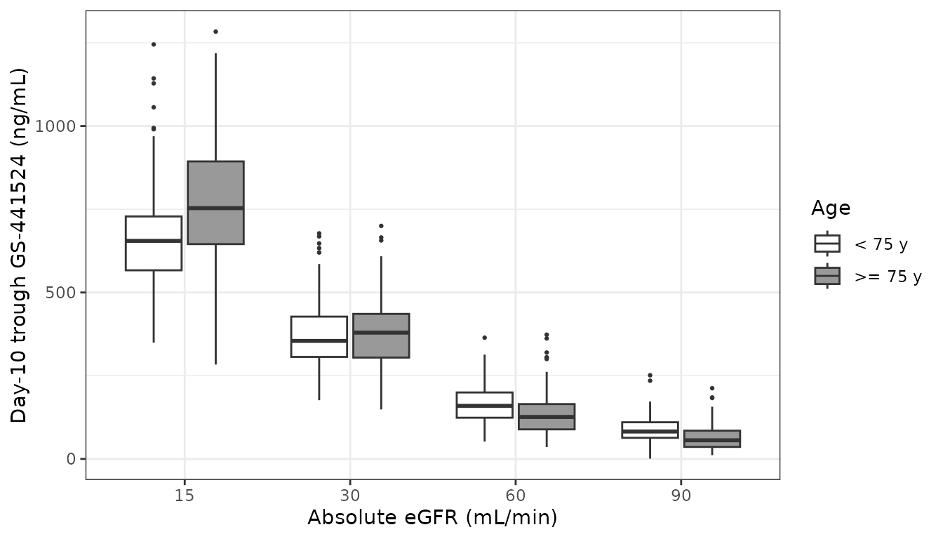
A cohort like the study (Figures 1a and 3)
This cohort is built to look like the study population and follows the package-insert regimen for 10 days. Patients are split across the three renal bands in the published proportions at the start of therapy: 20, 15 and 2 of 37 at absolute eGFR >= 60, 30-60 and < 30 mL/min. Within each band, eGFR is drawn uniformly, bounded by the observed 16.4-147.7 mL/min range. The cohort median is therefore lower than the Table 1 median of 74.7 mL/min. That median pools every measurement point, and renal function improved in several patients during therapy. Patients below 30 mL/min get the paper’s reduced regimen (100 mg every 2 days from day 3). Age and BSA are drawn around their published medians. Covariates are held constant in time.
N_COH <- 200L
draw_trunc <- function(n, draw, lo, hi) {
  x <- draw(n)
  while (any(bad <- x < lo | x > hi)) x[bad] <- draw(sum(bad))
  x
}
bands <- tibble::tribble(
  ~lo, ~hi, ~n_published,
  60, 147.7, 20L,
  30, 60, 15L,
  16.4, 30, 2L
)
band <- sample(seq_len(nrow(bands)), N_COH, replace = TRUE,
               prob = bands$n_published / sum(bands$n_published))
cohort <- tibble(
  id = seq_len(N_COH),
  egfr_abs = runif(N_COH, bands$lo[band], bands$hi[band]),
  BSA = draw_trunc(N_COH, function(n) rnorm(n, 1.8, 0.18), 1.24, 2.21),
  AGE = draw_trunc(N_COH, function(n) rnorm(n, 72, 12), 45, 97)
) |>
  mutate(CRCL = egfr_abs * 1.73 / BSA,
         reduced = egfr_abs < 30)
cohort |>
  summarise(median_egfr = median(egfr_abs),
            pct_ge60 = 100 * mean(egfr_abs >= 60),
            pct_30_60 = 100 * mean(egfr_abs >= 30 & egfr_abs < 60),
            pct_lt30 = 100 * mean(egfr_abs < 30),
            pct_age_ge75 = 100 * mean(AGE >= 75)) |>
  dplyr::rename("Median eGFR (mL/min)" = median_egfr,
                "% eGFR >= 60" = pct_ge60, "% eGFR 30-60" = pct_30_60,
                "% eGFR < 30" = pct_lt30, "% age >= 75" = pct_age_ge75) |>
knitr::kable(digits = 1, caption = "Simulated cohort covariates.")| Median eGFR (mL/min) | % eGFR >= 60 | % eGFR 30-60 | % eGFR < 30 | % age >= 75 |
|---|---|---|---|---|
| 67.3 | 52.5 | 41 | 6.5 | 40 |
coh_doses <- function(reduced) {
  tt <- if (reduced) c(0, seq(48, 216, by = 48)) else seq(0, 216, by = 24)
  tibble(time = tt, amt = c(200, rep(100, length(tt) - 1)), dur = 1,
         evid = 1L, cmt = "central")
}
coh_obs <- tibble(time = sort(unique(c(seq(0, 240, by = 2), seq(24, 240, by = 24)))),
                  amt = NA_real_, dur = NA_real_, evid = 0L, cmt = "central")
coh_events <- cohort |>
  rowwise() |>
  do(bind_rows(coh_doses(.$reduced), coh_obs) |>
       mutate(id = .$id, CRCL = .$CRCL, BSA = .$BSA, AGE = .$AGE,
              reduced = .$reduced)) |>
  ungroup() |>
  arrange(id, time, desc(evid))

coh_sim <- rxode2::rxSolve(ui, coh_events, keep = "reduced",
                           returnType = "data.frame")
Replicates the layout of Figure 3 of Sukeishi 2022: simulated concentrations over the first 10 days (median and 90% interval, residual error included). The paper’s observations are troughs only, so the published pcVPC covers only the lower edge of this band.
coh_sim |>
  group_by(time) |>
  summarise(q05 = quantile(sim, 0.05), q50 = median(sim),
            q95 = quantile(sim, 0.95), .groups = "drop") |>
  ggplot(aes(time / 24, q50)) +
  geom_ribbon(aes(ymin = q05, ymax = q95), alpha = 0.25) +
  geom_line() +
  labs(x = "Time after first dose (days)", y = "GS-441524 (ng/mL)") +
  theme_bw()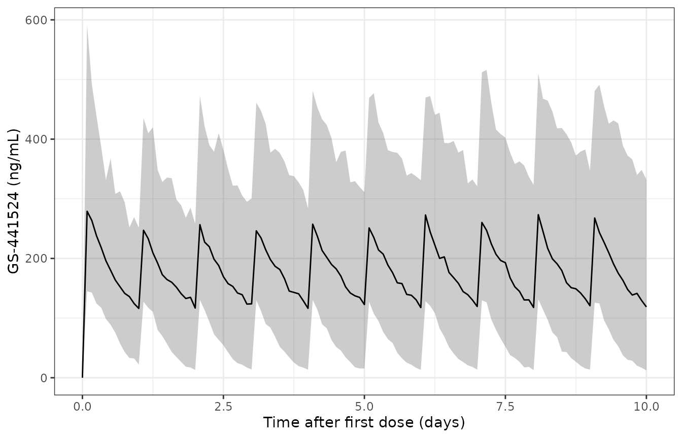
Troughs after day 4 are compared with the paper’s median observed concentration (116.6 ng/mL; the Results give the same value for the steady-state troughs after day 4).
coh_trough <- coh_sim |>
  filter(time %in% seq(120, 240, by = 24)) |>
  filter(!reduced | time %in% seq(144, 240, by = 48))
coh_med <- median(coh_trough$sim)
c(simulated_median_trough = coh_med, published = 116.6)
#> simulated_median_trough               published
#>                114.2913                116.6000

# The cohort covariates are assumptions, so the band is wide (83-163 ng/mL).
# Measured 114 / 93 / 118 ng/mL across three seeds. A lost MW ratio (about
# 2.07-fold) still falls well outside it.
stopifnot(abs(log(coh_med / 116.6)) < log(1.4))
Assumptions and deviations
-
Dose basis. The main text never states that doses
were converted to GS-441524 equivalents. The Supporting Information
control stream does (
S1=(V/1000)/(291.3/602.6)), and Table 3 is reproduced only with that conversion. Without it every trough is about 107% too high. -
IIV scale. Table 2 reports IIV as CV% for an
exponential model. It is converted as
omega^2 = log(CV^2 + 1). The simulated 90% intervals cannot distinguish this fromomega^2 = CV^2, and the two differ by about 3%. -
Residual error. The 15.2 CV% proportional error is
used as
propSd = 0.152. - Table 3 trough times. Not stated in the paper. Regimens 1 and 2 match the day-10 pre-dose trough and regimen 3 the day-14 pre-dose trough, as shown above.
-
eGFR input. The model takes the canonical
BSA-indexed
CRCL(mL/min/1.73 m^2) plusBSA, and de-indexes internally as the authors did. In the source this covariate varied over time; the cohorts here hold it constant. - Screened covariates. Sex, height, body weight, BSA (directly), serum creatinine, creatinine clearance, AST, ALT, albumin, ECMO and mechanical ventilation were screened (Tables S1-S2) and not retained. An alternative model with serum creatinine, height and age on CL (OBJ 1474) was rejected in favour of the eGFR model “considering clinical usefulness”. Its estimates are not published, so it is not included.
- Scope. The data are troughs only, and remdesivir itself was not measured, so the model does not describe the post-infusion peak of GS-441524 formation. Apply it to trough-level exposure.
- Figure 4 medians. The Figure 4 medians used in the age check were read off the published figure by eye by the maintainers (about +/- 20 ng/mL). They are used only in that check, never as parameter values.
- Study-like cohort. The eGFR, age and BSA distributions of the final cohort are reconstructed from the published renal-band counts and the Table 1 medians and ranges. They are not the patient-level data. The share of patients aged 75 or older is not reported; the age draw puts about 40% there.