Model and source
- Citation: Zhang L, Feng F, Wang X, Liang H, Yao X, Liu D. Dose Prediction and Pharmacokinetic Simulation of XZP-5610, a Small Molecule for NASH Therapy, Using Allometric Scaling and Physiologically Based Pharmacokinetic Models. Pharmaceuticals (Basel). 2024 Mar 13;17(3):369. doi:10.3390/ph17030369
- Description: One-compartment oral PK model for the non-steroidal FXR agonist XZP-5610 (NASH) in healthy Chinese adults, forward-predicted from SD rat and beagle dog preclinical PK by allometric scaling (Zhang 2024): first-order absorption from a depot with bioavailability, linear elimination from central. Every parameter is a cross-species prediction used for first-in-human dose selection, not an estimate fitted to human data; the paper reports no IIV and no residual error for it. The companion whole-body PBPK model in the same paper was built in PK-Sim v11.2 and is not reproducible from the published sources (no ODEs, organ volumes, blood flows, or per-tissue partition coefficients are reported).
- Article: https://doi.org/10.3390/ph17030369
- Supplement: https://www.mdpi.com/article/10.3390/ph17030369/s1
XZP-5610 is a non-steroidal, liver-selective farnesoid X receptor (FXR) agonist developed for non-alcoholic steatohepatitis (NASH). Zhang and colleagues combined in vitro ADME work, single-dose PK in SD rats and beagle dogs, and toxicology / pharmacodynamic studies to forward-predict the human PK parameters and the doses for the first-in-human (FIH) single ascending dose trial.
The paper contains two modelling layers:
- Allometric scaling (AS). Human intravenous clearance, steady-state volume of distribution, oral bioavailability and absorption rate constant were predicted from the rat and dog data. Together these four numbers define a one-compartment oral PK model, and it is that model which drives the paper’s dose calculations (Table 5). This is the model packaged here.
- Whole-body PBPK. A rat and a human PBPK model were built in PK-Sim v11.2 with Rodgers and Rowland tissue partitioning and the PK-Sim standard cellular permeability method, and were used to predict liver concentrations (Figure 4). This layer is not packaged – see Assumptions and deviations below.
Population
The model targets healthy Chinese adults enrolled in the FIH single ascending dose trial, dosed orally from 0.15 mg (the selected maximum recommended starting dose) up to 3 mg (the selected maximum dose). Per-cohort subject counts, ages, weights and sex balance for that trial are not reported in this paper; the clinical data appear only as predicted-versus-observed ratios in Figure 3. Allometric scaling assumed a single average adult body weight of 60 kg (Section 4.3.2), so no body-weight covariate enters the model.
None of the parameters was estimated from human data. They were forward-predicted from 24 SD rats (mean body weight 0.245 kg) and 24 beagle dogs (mean body weight 7.21 kg), each species split into one intravenous group and three single-dose oral groups (Section 4.3.1; PK in Tables 1 and 2). Human clearance was taken from the dog alone because rat hepatocyte metabolic stability differed markedly from human (Table S3: rat CL(liver) 42.3 vs human 12.6 mL/min/kg), which made the rat-derived human clearance roughly twofold too high (Section 2.4, Discussion).
The same information is available programmatically via the model’s
population metadata
(readModelDb("Zhang_2024_XZP5610")()$population).
Source trace
The per-parameter origin is recorded as an in-file comment next to
each ini() entry in
inst/modeldb/specificDrugs/Zhang_2024_XZP5610.R. The table
below collects them in one place, together with the arithmetic that
reproduces each published point value from the paper’s own tables.
| Equation / parameter | Value | Source location | Independent check |
|---|---|---|---|
lka (ka) |
1.46 /h | Section 2.4; Section 4.3.2 | mean(0.589, 2.34) = 1.4645, the dog and rat one-compartment NONMEM estimates that bound human ka |
lcl (CL) |
8.3 L/h | Section 2.4 (“138 mL/min (8.3 L/h)”); Table 5 footnote; Table 6 (0.138 L/h/kg) | mean of the four beagle-dog rows of Table 3 = mean(96.4, 92.3, 181, 184) = 138.4 mL/min |
lvc (Vss) |
41.8 L | Section 2.4 | mean of the three human Vss rows of Table 3 = mean(17.1, 45.3, 63.0) = 41.8 L |
lfdepot (F) |
0.574 | Section 2.4; Table 5 footnote | mean of the six beagle-dog oral F values in Table 2 = mean(43.4, 82.9, 51.2, 38.2, 61.4, 67.1) = 57.37% |
d/dt(depot) <- -ka * depot |
n/a | Section 4.3.2: “one-compartment PK models were constructed using NONMEM … with mean blood concentration data obtained after oral administration” | – |
d/dt(central) <- ka * depot - kel * central |
n/a | Section 4.3.2 (as above); linear PK asserted in the Discussion | – |
f(depot) <- exp(lfdepot) |
n/a | Section 2.4 (oral bioavailability applied to the oral dose) | Table 5 HED column, reproduced below |
Cc <- 1000 * central / vc |
n/a | unit conversion only: states in mg, vc in L, so
central / vc is mg/L and 1 mg/L = 1000 ng/mL |
– |
| IIV, residual error | absent | not reported: no parameter was fitted to human concentrations | – |
mod <- readModelDb("Zhang_2024_XZP5610")

ka <- 1.46      # 1/h
cl <- 8.3       # L/h
vc <- 41.8      # L
fF <- 0.574     # unitless

kel <- cl / vc
c(ka = ka, cl = cl, vc = vc, F = fF, kel = kel)
#>         ka         cl         vc          F        kel
#>  1.4600000  8.3000000 41.8000000  0.5740000  0.1985646
Virtual cohort
The packaged model is deterministic: the paper reports no inter-individual variability and no residual error, because none of its parameters was fitted to human concentrations. A single typical-value profile per dose level is therefore the complete prediction, and simulating a stochastic cohort would only add noise that the source does not support.
The four dose levels below are those the paper simulated in Figure 4 (0.15, 0.5, 1 and 3 mg), which span the FIH single-ascending-dose range from the selected maximum recommended starting dose to the selected maximum dose.
doses <- c(0.15, 0.5, 1, 3)

obs_times <- sort(unique(c(seq(0, 6, by = 0.05), seq(6, 24, by = 0.25))))

make_arm <- function(dose, id) {
  dplyr::bind_rows(
    tibble::tibble(
      id = id, time = 0, amt = dose, evid = 1L, cmt = "depot"
    ),
    tibble::tibble(
      id = id, time = obs_times, amt = NA_real_, evid = 0L, cmt = "central"
    )
  ) |>
    dplyr::mutate(treatment = sprintf("%g mg", dose))
}

events <- dplyr::bind_rows(
  lapply(seq_along(doses), function(i) make_arm(doses[i], id = i))
)

stopifnot(!anyDuplicated(unique(events[, c("id", "time", "evid")])))
Simulation
sim <- rxode2::rxSolve(
  mod,
  events = events,
  keep = c("treatment")
) |>
  as.data.frame()

# The model has no random effects, so every subject is the typical individual.
stopifnot(dplyr::n_distinct(sim$id) == length(doses))
Replicate published figures
The paper does not print a human plasma concentration-time figure: Figure 3 is a predicted-versus-observed ratio plot for the clinical SAD data (no concentrations or times are given), and Figure 4 shows liver concentrations from the PBPK model. The panel below is therefore the plasma prediction of the packaged AS model at the four Figure 4 dose levels – the plasma profile that the liver figure sits on top of.
sim |>
  dplyr::mutate(
    treatment = factor(treatment, levels = sprintf("%g mg", doses))
  ) |>
  ggplot(aes(time, Cc, colour = treatment)) +
  geom_line(linewidth = 0.8) +
  scale_x_continuous(breaks = seq(0, 24, by = 4)) +
  labs(
    x = "Time (h)", y = "Plasma XZP-5610 (ng/mL)", colour = "Single oral dose",
    title = "Predicted plasma XZP-5610 at the Figure 4 dose levels",
    caption = paste(
      "Companion to Figure 4 of Zhang 2024, which shows the corresponding",
      "PBPK-predicted liver concentrations."
    )
  ) +
  theme_bw()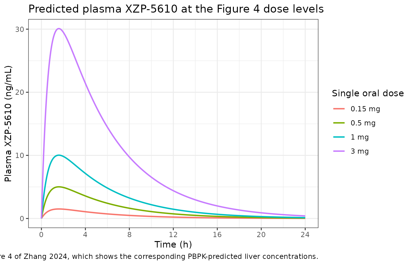
Zhang 2024 Section 2.7 reports that the PBPK model predicted human liver-to-plasma ratios of approximately 10.3 on Cmax and 13.5 on AUC. Applying those two published ratios to the plasma predictions above gives the liver exposures implied by Figure 4. These are annotations derived from the paper’s reported ratios, not outputs of the packaged model, which has no liver compartment.
liver_ratio_cmax <- 10.3   # Section 2.7
liver_ratio_auc  <- 13.5   # Section 2.7

tibble::tibble(
  treatment = sprintf("%g mg", doses),
  plasma_cmax = fF * doses / vc * (ka / (ka - kel)) *
    (exp(-kel * log(ka / kel) / (ka - kel)) -
       exp(-ka * log(ka / kel) / (ka - kel))) * 1000,
  plasma_auc = fF * doses / cl * 1000
) |>
  dplyr::mutate(
    liver_cmax = plasma_cmax * liver_ratio_cmax,
    liver_auc  = plasma_auc * liver_ratio_auc
  ) |>
  dplyr::rename(
    "Single oral dose"             = treatment,
    "Plasma Cmax (ng/mL)"          = plasma_cmax,
    "Plasma AUC0-inf (ng*h/mL)"    = plasma_auc,
    "Implied liver Cmax (ng/g)"    = liver_cmax,
    "Implied liver AUC0-inf (ng*h/g)" = liver_auc
  ) |>
  knitr::kable(
    digits = 2,
    caption = paste(
      "Liver exposure implied by the packaged plasma model and the",
      "liver-to-plasma ratios reported in Zhang 2024 Section 2.7",
      "(10.3 on Cmax, 13.5 on AUC). Annotation only; the packaged model",
      "has no liver compartment."
    )
)| Single oral dose | Plasma Cmax (ng/mL) | Plasma AUC0-inf (ng*h/mL) | Implied liver Cmax (ng/g) | Implied liver AUC0-inf (ng*h/g) |
|---|---|---|---|---|
| 0.15 mg | 1.50 | 10.37 | 15.50 | 140.04 |
| 0.5 mg | 5.02 | 34.58 | 51.66 | 466.81 |
| 1 mg | 10.03 | 69.16 | 103.32 | 933.61 |
| 3 mg | 30.09 | 207.47 | 309.96 | 2800.84 |
PKNCA validation
sim_nca <- sim |>
  dplyr::filter(!is.na(Cc)) |>
  dplyr::select(id, time, Cc, treatment)

# Guarantee a time = 0 record per subject; Cc = 0 pre-dose is correct for an
# extravascular single dose.
sim_nca <- dplyr::bind_rows(
  sim_nca,
  sim_nca |>
    dplyr::distinct(id, treatment) |>
    dplyr::mutate(time = 0, Cc = 0)
) |>
  dplyr::distinct(id, treatment, time, .keep_all = TRUE) |>
  dplyr::arrange(id, treatment, time)

conc_obj <- PKNCA::PKNCAconc(sim_nca, Cc ~ time | treatment + id)

dose_df <- events |>
  dplyr::filter(evid == 1L) |>
  dplyr::select(id, time, amt, treatment)

dose_obj <- PKNCA::PKNCAdose(dose_df, amt ~ time | treatment + id)

intervals <- data.frame(
  start      = 0,
  end        = Inf,
  cmax       = TRUE,
  tmax       = TRUE,
  aucinf.obs = TRUE,
  half.life  = TRUE
)

nca_res <- PKNCA::pk.nca(PKNCA::PKNCAdata(conc_obj, dose_obj,
                                          intervals = intervals))
Comparison against the closed-form one-compartment solution
The paper reports no numeric human NCA table (Cmax, Tmax, AUC and half-life for the clinical SAD cohorts appear only as ratios in Figure 3), so there is no published NCA to compare against directly. The available check on the packaged model is instead the analytic solution of the one-compartment oral model it encodes – an independent test of the numerically integrated ODEs and of the NCA itself, since the two routes share no code:
tmax_analytic <- log(ka / kel) / (ka - kel)

conc_analytic <- function(dose, t) {
  1000 * fF * dose * ka / (vc * (ka - kel)) * (exp(-kel * t) - exp(-ka * t))
}

analytic <- tibble::tibble(
  treatment  = sprintf("%g mg", doses),
  cmax       = conc_analytic(doses, tmax_analytic),
  tmax       = tmax_analytic,
  aucinf.obs = 1000 * fF * doses / cl,
  half.life  = log(2) / kel
)

cmp <- nlmixr2lib::ncaComparisonTable(
  simulated = nca_res,
  reference = analytic,
  by        = "treatment",
  units     = c(cmax = "ng/mL", tmax = "h",
                aucinf.obs = "ng*h/mL", half.life = "h"),
  tolerance_pct = 20
)

knitr::kable(
  cmp,
  digits  = 3,
  caption = paste(
    "PKNCA on the simulated profiles versus the closed-form one-compartment",
    "oral solution. * marks a >20% difference."
  )
)| NCA parameter | treatment | Reference | Simulated | % diff |
|---|---|---|---|---|
| Cmax (ng/mL) | 0.15 mg | 1.5 | 1.5 | -0.0% |
| Cmax (ng/mL) | 0.5 mg | 5.02 | 5.02 | -0.0% |
| Cmax (ng/mL) | 1 mg | 10 | 10 | -0.0% |
| Cmax (ng/mL) | 3 mg | 30.1 | 30.1 | -0.0% |
| Tmax (h) | 0.15 mg | 1.58 | 1.6 | +1.2% |
| Tmax (h) | 0.5 mg | 1.58 | 1.6 | +1.2% |
| Tmax (h) | 1 mg | 1.58 | 1.6 | +1.2% |
| Tmax (h) | 3 mg | 1.58 | 1.6 | +1.2% |
| AUC0-∞ (obs) (ng*h/mL) | 0.15 mg | 10.4 | 10.4 | -0.0% |
| AUC0-∞ (obs) (ng*h/mL) | 0.5 mg | 34.6 | 34.6 | -0.0% |
| AUC0-∞ (obs) (ng*h/mL) | 1 mg | 69.2 | 69.2 | -0.0% |
| AUC0-∞ (obs) (ng*h/mL) | 3 mg | 207 | 207 | -0.0% |
| t½ (h) | 0.15 mg | 3.49 | 3.51 | +0.5% |
| t½ (h) | 0.5 mg | 3.49 | 3.51 | +0.5% |
| t½ (h) | 1 mg | 3.49 | 3.51 | +0.5% |
| t½ (h) | 3 mg | 3.49 | 3.51 | +0.5% |
# Hard gate: the numerical simulation plus PKNCA must agree with the analytic
# solution to well within 5% on every parameter and every dose level.
nca_wide <- as.data.frame(nca_res) |>
  dplyr::select(treatment, PPTESTCD, PPORRES) |>
  tidyr::pivot_wider(names_from = PPTESTCD, values_from = PPORRES)

chk <- dplyr::inner_join(
  nca_wide, analytic,
  by = "treatment", suffix = c("_sim", "_ana")
) |>
  dplyr::mutate(
    dev_cmax  = abs(cmax_sim / cmax_ana - 1),
    dev_tmax  = abs(tmax_sim - tmax_ana),
    dev_auc   = abs(aucinf.obs_sim / aucinf.obs_ana - 1),
    dev_thalf = abs(half.life_sim / half.life_ana - 1)
  )

stopifnot(
  all(chk$dev_cmax  < 0.05),
  all(chk$dev_auc   < 0.05),
  all(chk$dev_thalf < 0.05),
  # Tmax is read off a 0.05 h observation grid, so compare on the grid scale.
  all(chk$dev_tmax  <= 0.05)
)

chk |>
  dplyr::select(treatment, dev_cmax, dev_auc, dev_thalf, dev_tmax) |>
  dplyr::rename(
    "Single oral dose"                  = treatment,
    "Cmax abs. deviation (fraction)"    = dev_cmax,
    "AUC0-inf abs. deviation (fraction)" = dev_auc,
    "t1/2 abs. deviation (fraction)"    = dev_thalf,
    "Tmax abs. deviation (h)"           = dev_tmax
  ) |>
  knitr::kable(
    digits  = 5,
    caption = "Simulation + PKNCA versus the analytic solution: deviations."
)| Single oral dose | Cmax abs. deviation (fraction) | AUC0-inf abs. deviation (fraction) | t1/2 abs. deviation (fraction) | Tmax abs. deviation (h) |
|---|---|---|---|---|
| 0.15 mg | 5e-05 | 1e-05 | 0.00546 | 0.01841 |
| 0.5 mg | 5e-05 | 1e-05 | 0.00546 | 0.01841 |
| 1 mg | 5e-05 | 1e-05 | 0.00546 | 0.01841 |
| 3 mg | 5e-05 | 1e-05 | 0.00546 | 0.01841 |
Dose proportionality
The Discussion asserts linear PK across the studied dose range. The packaged model is linear by construction, so this is a check that the simulation and NCA preserve that property rather than a test of the paper’s claim.
nca_wide |>
  dplyr::mutate(dose = doses[match(treatment, sprintf("%g mg", doses))]) |>
  dplyr::transmute(
    treatment,
    cmax_per_mg = cmax / dose,
    auc_per_mg  = aucinf.obs / dose,
    tmax,
    half.life
  ) |>
  dplyr::rename(
    "Single oral dose"             = treatment,
    "Cmax / dose (ng/mL per mg)"   = cmax_per_mg,
    "AUC0-inf / dose (ng*h/mL/mg)" = auc_per_mg,
    "Tmax (h)"                     = tmax,
    "t1/2 (h)"                     = half.life
  ) |>
  knitr::kable(
    digits  = 3,
    caption = "Dose-normalised NCA. Constant columns confirm dose linearity."
)| Single oral dose | Cmax / dose (ng/mL per mg) | AUC0-inf / dose (ng*h/mL/mg) | Tmax (h) | t1/2 (h) |
|---|---|---|---|---|
| 0.15 mg | 10.031 | 69.156 | 1.6 | 3.51 |
| 0.5 mg | 10.031 | 69.156 | 1.6 | 3.51 |
| 1 mg | 10.031 | 69.156 | 1.6 | 3.51 |
| 3 mg | 10.031 | 69.156 | 1.6 | 3.51 |
Reproducing Table 5 – the published human equivalent doses
Table 5 of Zhang 2024 converts each animal’s NOAEL steady-state
AUC0-24 into a human equivalent dose (HED) by free-fraction correction
followed by division by the predicted human CL/F. That second step uses
exactly the lcl and lfdepot values packaged
here, so recomputing the published HED and MRSD columns is a direct
numerical test of two of the model’s four parameters against printed
results.
The free-fraction ratio uses the values in the Table 5 footnote: fup is 1.3% in SD rat, 0.3% in beagle dog and 0.2% in human.
table5 <- tibble::tribble(
  ~species,      ~sex,      ~noael_mg_kg, ~auc_animal, ~fup_animal, ~auc_human_pub, ~hed_pub, ~mrsd_pub,
  "SD rat",      "Male",    1.5,          75.2,        0.013,       489,            7.07,     0.71,
  "SD rat",      "Female",  1.0,          46.4,        0.013,       302,            4.36,     0.44,
  "Beagle dog",  "Male",    0.05,         127.6,       0.003,       191,            2.77,     0.28,
  "Beagle dog",  "Female",  0.05,         152.1,       0.003,       228,            3.30,     0.33
)

fup_human <- 0.002   # Table 5 footnote and Table 6
safety_factor <- 10  # Section 2.5

table5_recomputed <- table5 |>
  dplyr::mutate(
    auc_human_calc = auc_animal * fup_animal / fup_human,
    # HED = AUC (ng*h/mL -> mg*h/L is /1000) * CL (L/h) / F
    hed_calc  = auc_human_pub / 1000 * cl / fF,
    mrsd_calc = hed_calc / safety_factor
  )

table5_recomputed |>
  dplyr::transmute(
    group = paste(species, sex),
    auc_human_pub, auc_human_calc,
    hed_pub, hed_calc,
    mrsd_pub, mrsd_calc
  ) |>
  dplyr::rename(
    "Species / sex"                 = group,
    "Human equiv AUC0-24, published (ng*h/mL)" = auc_human_pub,
    "Human equiv AUC0-24, recomputed"          = auc_human_calc,
    "HED, published (mg)"                      = hed_pub,
    "HED, recomputed (mg)"                     = hed_calc,
    "MRSD, published (mg)"                     = mrsd_pub,
    "MRSD, recomputed (mg)"                    = mrsd_calc
  ) |>
  knitr::kable(
    digits  = 2,
    caption = paste(
      "Zhang 2024 Table 5 recomputed from the packaged CL (8.3 L/h) and",
      "F (0.574). The HED column is reproduced to within 1%; every recomputed",
      "MRSD rounds exactly to the published two-decimal value."
    )
)| Species / sex | Human equiv AUC0-24, published (ng*h/mL) | Human equiv AUC0-24, recomputed | HED, published (mg) | HED, recomputed (mg) | MRSD, published (mg) | MRSD, recomputed (mg) |
|---|---|---|---|---|---|---|
| SD rat Male | 489 | 488.80 | 7.07 | 7.07 | 0.71 | 0.71 |
| SD rat Female | 302 | 301.60 | 4.36 | 4.37 | 0.44 | 0.44 |
| Beagle dog Male | 191 | 191.40 | 2.77 | 2.76 | 0.28 | 0.28 |
| Beagle dog Female | 228 | 228.15 | 3.30 | 3.30 | 0.33 | 0.33 |
stopifnot(
  # Free-fraction correction step.
  all(abs(table5_recomputed$auc_human_calc /
            table5_recomputed$auc_human_pub - 1) < 0.01),
  # HED from the packaged CL and F.
  all(abs(table5_recomputed$hed_calc /
            table5_recomputed$hed_pub - 1) < 0.01),
  # MRSD is published to two decimals, so compare on the published precision.
  # This is exact agreement, not a tolerance: every recomputed MRSD rounds to
  # the printed value.
  all(round(table5_recomputed$mrsd_calc, 2) == table5_recomputed$mrsd_pub)
)
Every published HED in Table 5 is reproduced to within 1% from the
packaged lcl and lfdepot, and every recomputed
MRSD rounds exactly to the published two-decimal value. Note that
although the supplementary equation (11) describes the divisor as the
animal bioavailability Fa, only the predicted
human bioavailability of 57.4% reproduces the printed HED
column; the Table 5 footnote states the same value. This is recorded
under Assumptions and deviations.
Safety margin at the selected FIH doses
The selected starting dose was 0.15 mg and the selected maximum dose 3 mg (Discussion). The model’s predicted exposures can be placed against the lowest human equivalent AUC derived from an animal NOAEL.
auc_per_mg <- 1000 * fF / cl                       # ng*h/mL per mg
lowest_noael_human_auc <- min(table5$auc_human_pub)  # ng*h/mL, beagle dog male

tibble::tibble(
  dose = c(0.15, 2, 3),
  role = c("selected MRSD", "selected MABEL", "selected MTD / max SAD dose"),
  auc  = dose * auc_per_mg
) |>
  dplyr::mutate(margin = lowest_noael_human_auc / auc) |>
  dplyr::rename(
    "Dose (mg)"                              = dose,
    "Role in the FIH design"                 = role,
    "Predicted AUC0-inf (ng*h/mL)"           = auc,
    "Fold below the lowest NOAEL-derived human AUC" = margin
  ) |>
  knitr::kable(
    digits  = 2,
    caption = paste(
      "Predicted single-dose exposures at the doses selected in Section 2.5",
      "versus the lowest animal-NOAEL-derived human equivalent AUC0-24",
      "(191 ng*h/mL, male beagle dog; Table 5)."
    )
)| Dose (mg) | Role in the FIH design | Predicted AUC0-inf (ng*h/mL) | Fold below the lowest NOAEL-derived human AUC |
|---|---|---|---|
| 0.15 | selected MRSD | 10.37 | 18.41 |
| 2.00 | selected MABEL | 138.31 | 1.38 |
| 3.00 | selected MTD / max SAD dose | 207.47 | 0.92 |
Assumptions and deviations
- The PBPK layer of the paper is not packaged. Zhang 2024 built rat and human whole-body PBPK models in PK-Sim v11.2 using the Rodgers and Rowland tissue partitioning method and the PK-Sim standard cellular-permeability method, and used them for Figures 2, 3 and 4. Reproducing that model in rxode2 requires the ODE system, the organ volumes and blood flows, and the per-tissue partition coefficients. None of these is reported. Table 6 lists only compound-level inputs (MW 556.46 g/mol; pKa 10.13 and 3.39; LogP 3.2; solubility 25 ug/mL at pH 6.0; Papp 10.1e-6 cm/s; fup 1.3% rat / 0.2% human; BP 0.58; CL 1.93 rat / 0.138 human L/h/kg; biliary clearance CLB 0.18) plus a single optimised liver-to-plasma partition coefficient KP,L = 37.0 and the names of the two calculation methods. The supplement (retrieved and read: it holds the hepatic-clearance and allometric-scaling equations plus Tables S1-S6 and Figure S1) contains no physiology either, and no PK-Sim project file was deposited. Per the PBPK / QSP sourcing rule, physiologic parameters are not substituted from platform defaults or class knowledge, so this layer is documented rather than guessed at.
-
No inter-individual variability and no residual
error. The four packaged parameters are cross-species
predictions, not estimates; the paper reports no variance components for
them, and none is invented here. Consequently the model simulates a
single typical profile per dose and
zeroRe()is unnecessary. -
All four parameters are wrapped in
fixed(). None was estimated. Each is a point prediction the authors held constant when computing the FIH doses. -
kais a cross-species average, not a human estimate. Section 4.3.2 fits one-compartment NONMEM models to rat and dog mean oral profiles and uses their ka estimates as the bounds of human ka; the packaged value 1.46 /h is the midpoint of that 0.589-2.34 /h range. The paper itself notes the animal-to-human correlation for ka is weak. -
Vssis used as the central volume. For a one-compartment model Vss and Vc coincide. The paper predicts only Vss and does not report a distributional phase for humans. -
Table 5’s divisor is human, not animal,
bioavailability. Supplementary equation (11) writes
Faand glosses it as “animal bioavailability”, but only F = 57.4% (the predicted human value, taken from the dog) reproduces the printed HED column; using the per-species animal F does not. The Table 5 footnote defines F as 57.4%. The printed table is treated as authoritative over the supplement’s gloss, and the vignette check above confirms the agreement to within 1%. - The clinical SAD data are not reproduced. Figure 3 reports only predicted/observed ratios; no concentrations, times or NCA values from the FIH trial are printed, so no observed-data overlay or published-NCA comparison is possible. The closed-form check above validates the packaged implementation, not the paper’s predictive accuracy.
- Rat and dog PK are not packaged as separate models. Tables 1 and 2 report non-compartmental CL, Vss and F for each species, and Section 4.3.2 reports a one-compartment NONMEM fit per species – but only ka was published from those fits. Building species models would require pairing the published ka with NCA-derived CL and Vss, a combination the authors never reported; in the rat that pairing implies a half-life of about 0.3 h against an observed 1.0-2.9 h, confirming that the rat is not one-compartment. Those tables therefore appear here as source-trace provenance only.
- Liver concentrations are annotations, not model output. The implied liver exposures shown above are the packaged plasma predictions multiplied by the liver-to-plasma ratios the paper reports in Section 2.7 (10.3 on Cmax, 13.5 on AUC). The packaged model has no liver compartment.
- Non-paper-derived parameter values: none. Every value in the model file is printed in the paper’s text or tables, and each is independently re-derived from a second location in the paper in the Source trace table above.