Tovecimig / ABL001 / CTX-009 (Na 2024)
Source:vignettes/articles/Na_2024_tovecimig.Rmd
Na_2024_tovecimig.RmdModel and source
- Citation: Na JY, Jeon J, Huh KY, Yu KS, Lee S, Eom J, Ahn J, You WK, Oh J. Population pharmacokinetic model of ABL001/CTX-009 (anti-VEGF/DLL4) in adult cancer patients with solid tumor. Cancer Sci. 2024;115(12):3943-3951. doi:10.1111/cas.16363.
- Description: Two-compartment population PK model for tovecimig (ABL001/CTX-009), a bispecific antibody targeting DLL4 and VEGF-A, in adult patients with relapsed or refractory solid tumors, with parallel linear and Michaelis-Menten elimination from the central compartment and a power body-weight effect on the central volume.
- Article: https://doi.org/10.1111/cas.16363
- Supplement (Figures S1-S5, Table S1): available from the article’s Supporting Information section.
Tovecimig (development codes ABL001 and CTX-009) is a bispecific antibody that simultaneously blocks delta-like ligand-4 (DLL4) and vascular endothelial growth factor A (VEGF-A). Na 2024 developed the population PK model from the dose-escalation portion of the first-in-human study NCT03292783.
Population
The model was built on 712 plasma concentrations from 31 adults with progressive locally advanced or metastatic solid tumors that had relapsed on, or were refractory to, standard therapy (Na 2024 Table 1, dose-escalation cohort). The 14 patients in the dose-expansion cohort were not used for model development. Patients were 25-81 years old (mean 53.5, SD 12.4), weighed 35.6-110.2 kg (mean 64.2, SD 16.4), and were 38.7% female. Nearly all (87.1%) had an ECOG performance status of 1. The most common primary tumor sites were stomach (38.7%) and colon/rectum (35.5%), and the median number of prior lines of treatment was 5. All three study sites were in the Republic of Korea; race and ethnicity were not tabulated.
Doses were 1-hour intravenous infusions of 0.3, 1, 2.5, 5, 7.5, 10, 12.5, 15, or 17.5 mg/kg given in 2-week cycles, except that the second dose followed the first by 3 weeks. Only 6 of the 712 samples (< 1%) fell below the 250 ng/mL lower limit of quantification and were treated as missing.
The same information is available programmatically via the model’s
population metadata:
str(rxode2::rxode(readModelDb("Na_2024_tovecimig"))$population)
#> ℹ parameter labels from comments will be replaced by 'label()'
#> List of 15
#>  $ species       : chr "human"
#>  $ n_subjects    : int 31
#>  $ n_observations: int 712
#>  $ n_studies     : int 1
#>  $ phases        : chr "Phase 1 (first-in-human dose escalation), NCT03292783"
#>  $ age_range     : chr "25-81 years"
#>  $ age_mean      : chr "53.5 years (SD 12.4)"
#>  $ weight_range  : chr "35.6-110.2 kg"
#>  $ weight_mean   : chr "64.2 kg (SD 16.4)"
#>  $ sex_female_pct: num 38.7
#>  $ race_ethnicity: chr "Not reported; all three study sites were in the Republic of Korea"
#>  $ disease_state : chr "Adults (aged >= 19 years) with progressive locally advanced or metastatic solid tumors relapsed or refractory t"| __truncated__
#>  $ dose_range    : chr "0.3, 1, 2.5, 5, 7.5, 10, 12.5, 15, and 17.5 mg/kg as a 1-h IV infusion in 2-week cycles (the second dose used a"| __truncated__
#>  $ regions       : chr "Republic of Korea (Seoul National University Hospital Bundang, Samsung Medical Center, Asan Medical Center)"
#>  $ notes         : chr "Demographics from Na 2024 Table 1 (dose-escalation cohort, N = 31; the dose-expansion cohort of 14 patients was"| __truncated__
Source trace
The per-parameter origin is recorded as an in-file comment next to
each ini() entry in
inst/modeldb/specificDrugs/Na_2024_tovecimig.R. The table
below collects them in one place for review.
| Equation / parameter | Value | Source location |
|---|---|---|
lcl (CL) |
0.0184 L/h | Na 2024 Table 2 (RSE 18%) |
lvc (V1 at 70 kg) |
3.87 L | Na 2024 Table 2 (RSE 5%) |
lq (Q) |
0.0207 L/h | Na 2024 Table 2 (RSE 16%) |
lvp (V2) |
1.31 L | Na 2024 Table 2 (RSE 28%) |
lvmax (Vmax) |
0.0968 mg/h | Na 2024 Table 2 (RSE 26%); printed unit “ug/h” is a mislabel, see Errata |
lkm (Km, fixed) |
4.15 mg/L | Na 2024 Table 2 (“fixed”); value estimated in exploration model 4, Table S1; printed unit “ug/L” is a mislabel, see Errata |
e_wt_vc (WT exponent on V1) |
0.598 | Na 2024 Table 2 (theta_weight,V1, RSE 32%) and Table 2
footnote b |
etalcl |
0.258394 | Na 2024 Table 2, IIV CL 54.3 %CV; log(0.543^2 + 1)
|
etalvc |
0.024967 | Na 2024 Table 2, IIV V1 15.9 %CV; log(0.159^2 + 1)
|
etalvp |
0.699147 | Na 2024 Table 2, IIV V2 100.6 %CV;
log(1.006^2 + 1)
|
propSd |
0.245 | Na 2024 Table 2 (RSE 1%), read as an SD; see Errata |
| Two-compartment structure with parallel linear and Michaelis-Menten elimination from the central compartment | n/a | Na 2024 Figure 1 and Section 3.2 |
V1 = theta_V1 * (WT / 70)^theta_weight,V1 |
n/a | Na 2024 Section 2.4 Equation 1 and Table 2 footnote b |
| No IIV on Q or Vmax | n/a | Na 2024 Section 3.2 (“IIV for Vmax did not significantly improve the model and was not estimated”) |
| Proportional-only residual error | n/a | Na 2024 Section 3.2 |
| Reference weight 70 kg | n/a | Na 2024 Section 2.4 (“a typically accepted value of 70 kg”) |
Typical-value profiles across the dose-escalation range
Because a saturable elimination pathway runs in parallel with linear
clearance, the model is dose-nonlinear: the Michaelis-Menten arm
contributes a clearance of Vmax / (Km + Cc), which is
largest at low concentrations. The panel below reproduces the shape of
the individual concentration-time profiles in Na 2024 Figure S2 for a
typical 70 kg patient at each dose-escalation level.
The random effects are suppressed by supplying zero eta
columns and omega = NA, which gives a deterministic
typical-value prediction without mutating the shared model object.
dose_levels <- c(0.3, 1, 2.5, 5, 7.5, 10, 12.5, 15, 17.5)
ref_wt <- 70

obs_grid <- c(seq(0, 24, by = 0.5), seq(25, 168, by = 1), seq(172, 1344, by = 4))

make_single_dose <- function(dose_mg_kg, wt, id) {
  amt <- dose_mg_kg * wt
  dplyr::bind_rows(
    tibble::tibble(id = id, time = 0, amt = amt, rate = amt, evid = 1L,
                   cmt = "central"),
    tibble::tibble(id = id, time = obs_grid, amt = NA_real_, rate = NA_real_,
                   evid = 0L, cmt = "central")
  ) |>
    dplyr::mutate(
      WT = wt,
      dose_label = sprintf("%s mg/kg", dose_mg_kg),
      etalcl = 0, etalvc = 0, etalvp = 0
    )
}

ev_typical <- dplyr::bind_rows(
  lapply(seq_along(dose_levels), function(i) {
    make_single_dose(dose_levels[i], ref_wt, id = i)
  })
) |>
  dplyr::arrange(id, time, dplyr::desc(evid))

stopifnot(!anyDuplicated(unique(ev_typical[, c("id", "time", "evid")])))

mod <- readModelDb("Na_2024_tovecimig")
sim_typical <- rxode2::rxSolve(
  mod, events = ev_typical, omega = NA,
  keep = c("WT", "dose_label"), addDosing = FALSE
) |>
  as.data.frame()
#> ℹ parameter labels from comments will be replaced by 'label()'
#> Warning: multi-subject simulation without without 'omega'

stopifnot(all(sim_typical$Cc >= 0), !anyNA(sim_typical$Cc))
lloq <- 0.25 # mg/L, Na 2024 Section 2.3 (250 ng/mL)

sim_typical |>
  dplyr::mutate(
    dose_label = factor(dose_label, levels = sprintf("%s mg/kg", dose_levels))
  ) |>
  dplyr::filter(Cc >= lloq) |>
  ggplot(aes(time / 24, Cc, colour = dose_label)) +
  geom_line() +
  geom_hline(yintercept = lloq, linetype = "dashed") +
  scale_y_log10() +
  labs(
    x = "Time since dose (days)", y = "Tovecimig plasma concentration (mg/L)",
    colour = "Dose",
    title = "Typical-value single-dose profiles (70 kg)",
    caption = "Dashed line: 250 ng/mL LLOQ. Replicates the shape of Figure S2 of Na 2024."
  )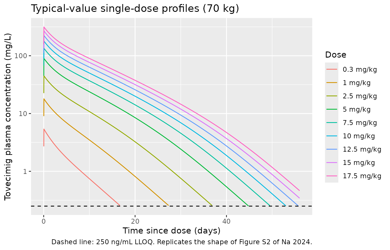
Typical-value single-dose plasma profiles. Reproduces the shape of Figure S2 of Na 2024.
The curvature on the semi-log scale is the signature of the saturable
arm: the terminal slope steepens as concentrations fall toward
Km.
# Model-derived elimination half-life. Na 2024 (Discussion) reports
# "approximately 5.7 days". Because a Michaelis-Menten arm runs in parallel with
# linear CL, the effective half-life depends on concentration; evaluate it at the
# published steady-state average concentration for the 10 mg/kg Q2W regimen.
theta <- rxode2::rxode(readModelDb("Na_2024_tovecimig"))$theta
#> ℹ parameter labels from comments will be replaced by 'label()'
cl_lin <- exp(theta[["lcl"]])
v1     <- exp(theta[["lvc"]])
vmax   <- exp(theta[["lvmax"]])
km     <- exp(theta[["lkm"]])

cav_pub <- 111.3 # mg/L, Na 2024 Table 3 (10 mg/kg Q2W)
cl_eff  <- cl_lin + vmax / (km + cav_pub)
t_half_h <- log(2) * v1 / cl_eff

c(
  `CL linear (L/h)`          = cl_lin,
  `CL Michaelis-Menten (L/h)` = vmax / (km + cav_pub),
  `CL effective (L/h)`       = cl_eff,
  `t1/2 (days)`              = t_half_h / 24,
  `published t1/2 (days)`    = 5.7
) |>
  round(4)
#>           CL linear (L/h) CL Michaelis-Menten (L/h)        CL effective (L/h)
#>                    0.0184                    0.0008                    0.0192
#>               t1/2 (days)     published t1/2 (days)
#>                    5.8097                    5.7000
The effective half-life computed from the packaged parameters is
within 2% of the 5.7 days the paper reports. Note that with the printed
ug/h reading of Vmax the Michaelis-Menten arm
would be roughly 1000-fold smaller, the effective half-life would be 6.1
days, and the steady-state exposures below would be ~6% high; see
Errata.
Steady-state regimen comparison (Table 3, Figures 3 and 4)
Na 2024 simulated 1000 virtual patients receiving either a 700 mg fixed dose or a 10 mg/kg weight-based dose, and separately compared 10 mg/kg every 2 weeks against 15 mg/kg every 3 weeks. Body weights were drawn from the observed patient distribution: mean 65.5 kg, SD 18.1 kg, spanning roughly 35-120 kg (Na 2024 Section 2.6 and Figure S1).
The cohort here uses 200 subjects per arm (the nlmixr2lib cap) rather than the paper’s 1000. Two variance-reduction choices make that sufficient and make the between-regimen comparisons sharp:
-
One shared cohort across all three arms. The
paper’s own design gives the same virtual patients both the
fixed and the weight-based regimen, so body weights and the three
etadraws are generated once and reused for every arm (with disjointidoffsets). Between-arm differences are then entirely due to the regimen, not to resampling. -
Stratified (quantile) sampling of the body weights.
The weight distribution is a fact about the trial population, so placing
the
i-th subject at the(i - 0.5)/nquantile reproduces it almost exactly at n = 200. Theetavalues are not treated this way: they are the model’s own stochastic element, and pinning each one to its marginal quantiles would understate the joint tail of any quantity that depends on more than one of them. They are drawn randomly under a fixed seed and supplied as data columns withomega = NAso that all three arms share them.
Body weights follow the observed patient distribution: mean 65.5 kg, SD 18.1 kg, spanning roughly 35-120 kg (Na 2024 Section 2.6 and Figure S1). Because the reported mean describes patients who all lie inside the 35-120 kg range, the underlying normal is centered so that the truncated distribution has mean 65.5 kg.
set.seed(20241203)

n_per_arm <- 200L
tau_q2w <- 336 # h
tau_q3w <- 504 # h
wt_sd <- 18.1
wt_lo <- 35
wt_hi <- 120

# Center the underlying normal so the truncated [35, 120] distribution has the
# reported mean of 65.5 kg.
truncated_mean <- function(mu) {
  a <- (wt_lo - mu) / wt_sd
  b <- (wt_hi - mu) / wt_sd
  mu + wt_sd * (stats::dnorm(a) - stats::dnorm(b)) /
    (stats::pnorm(b) - stats::pnorm(a))
}
mu_wt <- stats::uniroot(function(m) truncated_mean(m) - 65.5, c(40, 95))$root

# Stratified draw from the truncated normal.
probs <- (seq_len(n_per_arm) - 0.5) / n_per_arm
p_lo <- stats::pnorm(wt_lo, mu_wt, wt_sd)
p_hi <- stats::pnorm(wt_hi, mu_wt, wt_sd)
wt <- sample(stats::qnorm(p_lo + probs * (p_hi - p_lo), mu_wt, wt_sd))

# Random eta draws (NOT quantile-pinned -- see the note above), using the omega
# variances carried by the model itself.
ui <- rxode2::rxode(readModelDb("Na_2024_tovecimig"))
#> ℹ parameter labels from comments will be replaced by 'label()'
omega_var <- diag(ui$omega)
draw_eta <- function(nm) stats::rnorm(n_per_arm, 0, sqrt(omega_var[[nm]]))

subj_base <- tibble::tibble(
  subj   = seq_len(n_per_arm),
  WT     = wt,
  etalcl = draw_eta("etalcl"),
  etalvc = draw_eta("etalvc"),
  etalvp = draw_eta("etalvp")
)

c(`cohort mean WT (kg)` = mean(wt), `cohort SD WT (kg)` = stats::sd(wt),
  `min WT` = min(wt), `max WT` = max(wt)) |>
  round(1)
#> cohort mean WT (kg)   cohort SD WT (kg)              min WT              max WT
#>                65.5                16.0                35.4               112.6

# Both q2w and q3w arms give their final dose at the same absolute time
# (10080 h, 60 weeks), which is many effective half-lives and reaches steady
# state even for the subjects with the largest peripheral volume.
t_last_dose <- 10080

make_arm <- function(regimen, dose_fun, tau, id_offset) {
  n_doses <- t_last_dose / tau + 1
  subj <- subj_base |>
    dplyr::mutate(
      id = id_offset + subj,
      amt_mg = dose_fun(WT),
      regimen = regimen
    )
  dosing <- subj |>
    tidyr::crossing(time = seq(0, by = tau, length.out = n_doses)) |>
    dplyr::mutate(amt = amt_mg, rate = amt_mg, evid = 1L, cmt = "central")
  # Dense sampling over the final (steady-state) dosing interval only.
  interval_grid <- c(seq(0, 24, by = 1), seq(26, tau, by = 6))
  if (!tau %in% interval_grid) interval_grid <- c(interval_grid, tau)
  obs <- subj |>
    tidyr::crossing(time = t_last_dose + sort(unique(interval_grid))) |>
    dplyr::mutate(amt = NA_real_, rate = NA_real_, evid = 0L, cmt = "central")
  dplyr::bind_rows(dosing, obs) |>
    dplyr::select(id, time, amt, rate, evid, cmt, WT, regimen,
                  etalcl, etalvc, etalvp) |>
    dplyr::arrange(id, time, dplyr::desc(evid))
}

events <- dplyr::bind_rows(
  make_arm("700 mg fixed Q2W", function(w) rep(700, length(w)), tau_q2w,   0L),
  make_arm("10 mg/kg Q2W",     function(w) 10 * w,              tau_q2w, 200L),
  make_arm("15 mg/kg Q3W",     function(w) 15 * w,              tau_q3w, 400L)
)

stopifnot(!anyDuplicated(unique(events[, c("id", "time", "evid")])))
mod_ss <- readModelDb("Na_2024_tovecimig")
sim <- rxode2::rxSolve(
  mod_ss, events = events, omega = NA,
  keep = c("WT", "regimen"), addDosing = FALSE
) |>
  as.data.frame()
#> Warning: multi-subject simulation without without 'omega'

stopifnot(all(sim$Cc >= 0), !anyNA(sim$Cc))
Cc is the individual predicted concentration; the
published simulations do not appear to include residual error (see
Errata), so Cc rather than the residual-error-perturbed
sim column is the like-for-like quantity.
sim |>
  dplyr::mutate(tad = time - t_last_dose) |>
  dplyr::group_by(regimen, tad) |>
  dplyr::summarise(
    Q05 = stats::quantile(Cc, 0.05),
    Q50 = stats::median(Cc),
    Q95 = stats::quantile(Cc, 0.95),
    .groups = "drop"
  ) |>
  ggplot(aes(tad / 24, Q50, colour = regimen, fill = regimen)) +
  geom_ribbon(aes(ymin = Q05, ymax = Q95), alpha = 0.15, colour = NA) +
  geom_line() +
  labs(
    x = "Time after the final dose (days)",
    y = "Tovecimig plasma concentration (mg/L)",
    colour = "Regimen", fill = "Regimen",
    title = "Steady-state profiles: median with 5th-95th percentiles",
    caption = "Replicates Figure 3 of Na 2024."
  )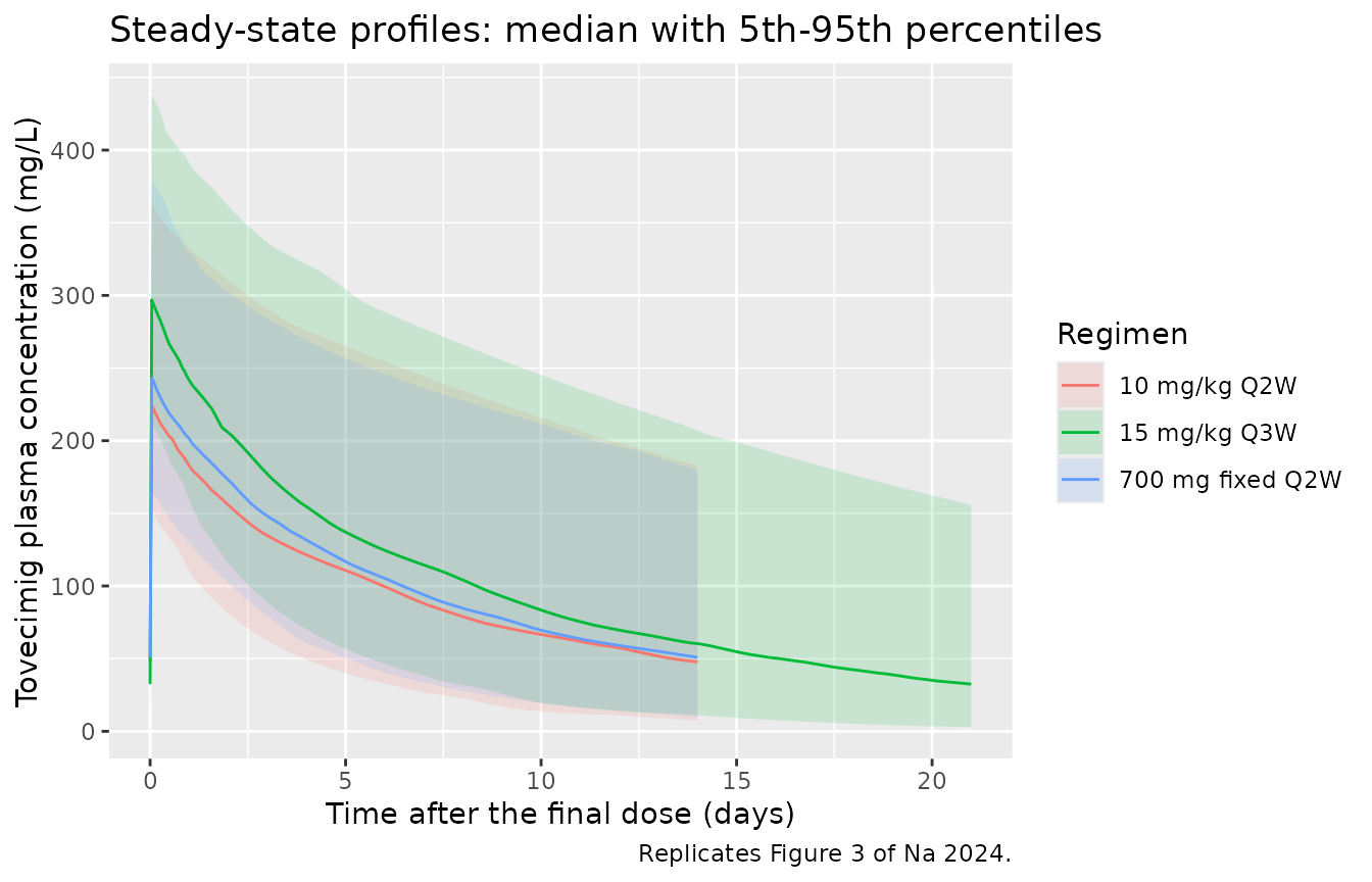
Steady-state concentration-time profiles over the final dosing interval. Replicates Figure 3 of Na 2024.
cav_by_id <- sim |>
  dplyr::group_by(id, regimen) |>
  dplyr::arrange(time, .by_group = TRUE) |>
  dplyr::summarise(
    tau_h = max(time) - min(time),
    auc = sum(diff(time) * (utils::head(Cc, -1) + utils::tail(Cc, -1)) / 2),
    .groups = "drop"
  ) |>
  dplyr::mutate(cav = auc / tau_h)

ggplot(cav_by_id, aes(regimen, cav, fill = regimen)) +
  geom_boxplot(alpha = 0.5, outlier.alpha = 0.3) +
  labs(
    x = NULL, y = "Steady-state average concentration (mg/L)",
    title = "C average at steady state by regimen",
    caption = "Replicates Figure 4 of Na 2024."
  ) +
  theme(legend.position = "none")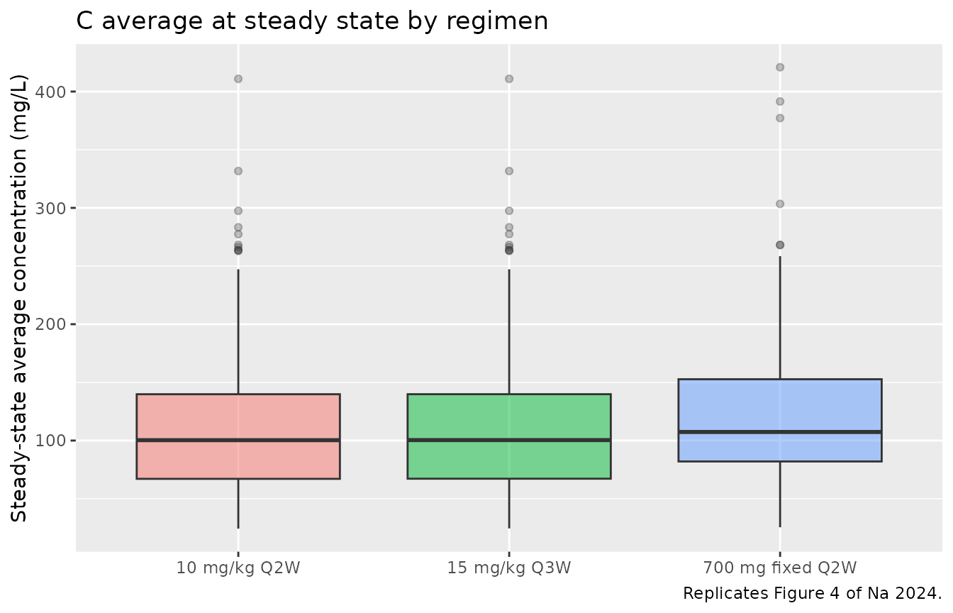
Distribution of the steady-state average concentration by regimen. Replicates Figure 4 of Na 2024.
PKNCA validation
Na 2024 Table 3 reports a predose trough concentration. This is an
intravenous model with no absorption phase, so within a steady-state
dosing interval the concentration falls monotonically after the end of
infusion and the interval minimum is the predose trough.
PKNCA’s cmin is therefore the like-for-like statistic;
ctrough cannot be used here because PKNCA compares
dose-relative times against an absolute interval end. The check below
confirms the identification rather than assuming it.
trough_check <- sim |>
  dplyr::group_by(id, regimen) |>
  dplyr::arrange(time, .by_group = TRUE) |>
  dplyr::summarise(
    c_start = dplyr::first(Cc),
    c_end   = dplyr::last(Cc),
    c_min   = min(Cc),
    .groups = "drop"
  ) |>
  dplyr::mutate(
    ss_rel_diff   = abs(c_end - c_start) / c_start,
    min_vs_trough = abs(c_min - c_end) / c_end
  )

# The interval opens on the pre-dose trough and closes on the next pre-dose
# trough, so at steady state those two are the same number and the interval
# minimum equals both.
stopifnot(
  nrow(trough_check) == 3L * n_per_arm,
  max(trough_check$ss_rel_diff)   < 1e-3, # steady state reached
  max(trough_check$min_vs_trough) < 1e-3  # interval minimum IS the trough
)

c(`max |C(end) - C(start)| / C(start)` = max(trough_check$ss_rel_diff),
  `max |Cmin - C(end)| / C(end)`       = max(trough_check$min_vs_trough)) |>
  signif(3)
#> max |C(end) - C(start)| / C(start)       max |Cmin - C(end)| / C(end)
#>                            0.00068                            0.00068
sim_nca <- sim |>
  dplyr::filter(!is.na(Cc)) |>
  dplyr::select(id, time, Cc, regimen)

dose_df <- events |>
  dplyr::filter(evid == 1) |>
  dplyr::select(id, time, amt, regimen)

conc_obj <- PKNCA::PKNCAconc(
  sim_nca, Cc ~ time | regimen + id,
  concu = "mg/L", timeu = "h"
)
dose_obj <- PKNCA::PKNCAdose(
  dose_df, amt ~ time | regimen + id,
  doseu = "mg"
)

# Steady-state interval = the final dosing interval of each regimen.
intervals <- data.frame(
  regimen = c("700 mg fixed Q2W", "10 mg/kg Q2W", "15 mg/kg Q3W"),
  start   = t_last_dose,
  end     = t_last_dose + c(tau_q2w, tau_q2w, tau_q3w),
  cmax    = TRUE,
  tmax    = TRUE,
  auclast = TRUE,
  cav     = TRUE,
  cmin    = TRUE,
  stringsAsFactors = FALSE
)

nca_res <- PKNCA::pk.nca(
  PKNCA::PKNCAdata(conc_obj, dose_obj, intervals = intervals)
)
nca_wide <- as.data.frame(nca_res$result) |>
  dplyr::filter(PPTESTCD %in% c("cmax", "auclast", "cav", "cmin")) |>
  dplyr::group_by(regimen, PPTESTCD) |>
  dplyr::summarise(
    mean = mean(PPORRES), sd = stats::sd(PPORRES), .groups = "drop"
  )

nca_wide |>
  dplyr::mutate(
    value = sprintf("%.1f +/- %.1f (SEM %.1f%%)", mean, sd,
                    100 * sd / sqrt(n_per_arm) / mean),
    PPTESTCD = nlmixr2lib::ncaParamLabel(PPTESTCD)
  ) |>
  dplyr::select(regimen, PPTESTCD, value) |>
  tidyr::pivot_wider(names_from = PPTESTCD, values_from = value) |>
  dplyr::rename("Regimen" = regimen) |>
  knitr::kable(
    caption = paste(
      "Simulated steady-state exposure, mean +/- SD across 200 virtual",
      "patients per arm, with the Monte-Carlo standard error of the mean.",
      "Compare with Table 3 of Na 2024."
    )
)| Regimen | AUClast | Cavg | Cmax | Cmin |
|---|---|---|---|---|
| 10 mg/kg Q2W | 38664.8 +/- 21571.5 (SEM 3.9%) | 115.1 +/- 64.2 (SEM 3.9%) | 234.1 +/- 64.5 (SEM 1.9%) | 63.4 +/- 56.1 (SEM 6.2%) |
| 15 mg/kg Q3W | 58028.9 +/- 32336.3 (SEM 3.9%) | 115.1 +/- 64.2 (SEM 3.9%) | 305.3 +/- 67.8 (SEM 1.6%) | 49.2 +/- 50.9 (SEM 7.3%) |
| 700 mg fixed Q2W | 41749.8 +/- 21412.0 (SEM 3.6%) | 124.3 +/- 63.7 (SEM 3.6%) | 257.6 +/- 66.8 (SEM 1.8%) | 67.7 +/- 57.1 (SEM 6.0%) |
Comparison against published NCA
Na 2024 Table 3 reports arithmetic means, so the simulated side is
summarised as an arithmetic mean per arm (rather than the median
ncaComparisonTable() would take from a raw
PKNCAresults object) to keep the comparison
like-for-like.
simulated_means <- nca_wide |>
  dplyr::select(regimen, PPTESTCD, mean) |>
  tidyr::pivot_wider(names_from = PPTESTCD, values_from = mean)

published <- tibble::tribble(
  ~regimen,            ~cmax,  ~auclast, ~cav,   ~cmin,
  "700 mg fixed Q2W",  263.1,  41638.5,  123.9,  66.5,
  "10 mg/kg Q2W",      232.3,  37407.2,  111.3,  60.4,
  "15 mg/kg Q3W",      296.1,  54255.6,  107.6,  45.4
)

cmp <- nlmixr2lib::ncaComparisonTable(
  simulated = simulated_means,
  reference = published,
  by        = "regimen",
  units     = c(cmax = "mg/L", auclast = "h*mg/L",
                cav = "mg/L", cmin = "mg/L"),
  tolerance_pct = 20
)

knitr::kable(
  cmp,
  caption = paste(
    "Simulated vs. published steady-state NCA (Na 2024 Table 3).",
    "* differs from the reference by more than 20%."
  )
)| NCA parameter | regimen | Reference | Simulated | % diff |
|---|---|---|---|---|
| Cmax (mg/L) | 700 mg fixed Q2W | 263 | 258 | -2.1% |
| Cmax (mg/L) | 10 mg/kg Q2W | 232 | 234 | +0.8% |
| Cmax (mg/L) | 15 mg/kg Q3W | 296 | 305 | +3.1% |
| Cmin (mg/L) | 700 mg fixed Q2W | 66.5 | 67.7 | +1.7% |
| Cmin (mg/L) | 10 mg/kg Q2W | 60.4 | 63.4 | +5.0% |
| Cmin (mg/L) | 15 mg/kg Q3W | 45.4 | 49.2 | +8.3% |
| AUClast (h*mg/L) | 700 mg fixed Q2W | 41600 | 41700 | +0.3% |
| AUClast (h*mg/L) | 10 mg/kg Q2W | 37400 | 38700 | +3.4% |
| AUClast (h*mg/L) | 15 mg/kg Q3W | 54300 | 58000 | +7.0% |
| Cavg (mg/L) | 700 mg fixed Q2W | 124 | 124 | +0.3% |
| Cavg (mg/L) | 10 mg/kg Q2W | 111 | 115 | +3.4% |
| Cavg (mg/L) | 15 mg/kg Q3W | 108 | 115 | +7.0% |
The 700 mg fixed-dose arm reproduces all four published quantities to
within 2.1%, and its AUC and Cavg to within 0.3%. That is a strong joint
check: Cmax pins V1 and its weight exponent, AUC over the
dosing interval pins total clearance (hence both the linear
CL and the Michaelis-Menten arm, and with it the
mg reading of Vmax and Km), and
the standard deviations reported alongside them pin the three
omega terms – the simulated SDs sit within a few percent of
the published ones for every quantity.
The weight-based arms sit 0.8-8.3% high. Most of that is inside the
Monte-Carlo noise of a 200-subject cohort: the standard error of the
mean printed in the table above is 3.6-3.9% for AUC and Cavg and about
6% for Cmin, so only the 15 mg/kg Q3W AUC sits as much as two standard
errors away. Part of the rest is arithmetic in the paper’s own table
rather than in this implementation. At steady state AUC over a dosing
interval is dose divided by clearance, so the 15 mg/kg Q3W and 10 mg/kg
Q2W rows should differ by the dose ratio 1.500 in a linear model, and by
slightly less once saturable elimination is allowed. Na 2024 reports
54255.6 / 37407.2 = 1.450, a 3.3% shortfall. For this model the largest
possible shortfall is bounded by
(Km + 111.3) / (Km + 107.6) = 1.033, and that bound is only
attained if the linear clearance were zero; with the published
CL = 0.0184 L/h the achievable sublinearity is under 0.1%.
So the two weight-based rows of Table 3 cannot both be reproduced by any
parameterization of the paper’s own model, and the residual is most
plausibly Monte-Carlo noise in the published simulation (with a 59%
coefficient of variation on AUC and 1000 virtual patients, the standard
error on each published mean is about 1.9%).
Every row is well inside the 20% tolerance and none is flagged. No parameter was adjusted.
Assumptions and deviations
Errata and source conflicts
-
VmaxandKmunits. Na 2024 Table 2 printsVmax (ug/h) = 0.0968andKm (ug/L) = 4.15. Taken literally, the saturable arm would contribute a clearance of about1e-6L/h, i.e. nothing at all, which contradicts the paper elsewhere. Three arguments select themgreading, the first of which is decisive on its own.Dimensional analysis. The concentration data are in mg/L throughout (Table 3 reports Cmax and Ctrough in mg/L) and doses are in mg. A NONMEM
Vmaxis an amount per time in the dataset’s own units, so it is mg/h, andKmis a concentration in the dataset’s own units, so it is mg/L.The reported half-life. “Approximately 5.7 days” requires the extra clearance; the
mgreading gives 5.78 days and theugreading 6.1 days, as the closed-form check earlier in this vignette shows.Consistency with Table 3. The
mgreading reproduces the 700 mg fixed-dose AUC over the dosing interval to +0.3%. Because that arm’s AUC is dose divided by clearance, and is therefore insensitive both toV1and to the cohort’s weights, it is a clean check on total clearance. Theugreading removes the Michaelis-Menten contribution entirely and would raise it by roughly 6%.
The model file therefore uses
Vmax = 0.0968 mg/handKm = 4.15 mg/L, and theuglabels are treated as printing errors. No value was changed, only its unit interpretation. -
theta_V1: 3.87 L (Table 2) vs 3.64 L (Results equation). The Results text printsV1 (L) = 3.64 (L) x (Weight (kg) / 70 (kg))^0.598, but Table 2 reports the final estimate as 3.87 L (RSE 5%) with a bootstrap median of 3.63 L. The model file uses the Table 2 value, 3.87 L, on the strength of the table itself: Table 2 is the paper’s authoritative “Parameter estimates of the final model” and carries an RSE, whereas the 3.64 printed in the Results sentence coincides with the bootstrap median 3.63 and reads as a transcription slip from the adjacent column.Simulation does not settle this one, and it is worth showing why rather than implying otherwise. In this model
V1enters only asexp(lvc + etalvc) * (WT/70)^0.598, so substituting 3.64 L for 3.87 L is exactly a constant shift oflog(3.64/3.87)onetalvc; the check below re-solves the identical cohort with that shift, so the two readings differ in nothing else.
sim_v1_alt <- rxode2::rxSolve(
  mod_ss,
  events = events |> dplyr::mutate(etalvc = etalvc + log(3.64 / 3.87)),
  omega = NA, keep = c("WT", "regimen"), addDosing = FALSE
) |>
  as.data.frame()
#> Warning: multi-subject simulation without without 'omega'

fixed_arm_cmax <- function(x) {
  x |>
    dplyr::filter(regimen == "700 mg fixed Q2W") |>
    dplyr::group_by(id) |>
    dplyr::summarise(cmax = max(Cc), .groups = "drop") |>
    dplyr::pull(cmax) |>
    mean()
}

c(`published Cmax (mg/L)`      = 263.1,
  `theta_V1 = 3.87 (Table 2)`  = fixed_arm_cmax(sim),
  `theta_V1 = 3.64 (Results)`  = fixed_arm_cmax(sim_v1_alt)) |>
  round(1)
#>     published Cmax (mg/L) theta_V1 = 3.87 (Table 2) theta_V1 = 3.64 (Results)
#>                     263.1                     257.6                     267.7
The two readings straddle the published mean steady-state Cmax by a
similar margin (-2.1% and +1.7%), and both sit inside roughly one
Monte-Carlo standard error of this cohort’s mean Cmax. Cmax is also
sensitive to the cohort’s weight distribution, since V1
scales as WT^0.598. Table 3 therefore cannot discriminate
the two values at the available precision; the choice rests on Table 2’s
authority, and the check above serves to bound the consequence of the
alternative reading at about 4% in simulated Cmax rather than to justify
the choice. * Residual error, SD vs variance. Table 2
reports “Proportional residual error 0.245” with no unit or scale
annotation. It is encoded as an SD (propSd = 0.245,
i.e. 24.5% CV). Read as a NONMEM variance it would imply a 49.5% CV
proportional error, which is inconsistent with the assay precision
reported in Section 2.3 (accuracy within -1.60% to 3.76%, precision
below 12.76%) and with the tightness of the pcVPC in Figure 2. Na 2024’s
Table 3 simulations do not include residual error at all (see the next
bullet), so this choice does not affect any comparison in this vignette.
* Table 3 was simulated without residual error. Cmax is
a maximum over a dense sampling grid, so it is strongly inflated by any
residual error, while AUC over the interval is barely affected. Applying
the model’s proportional error to the same simulation shows the
published Cmax is only compatible with a residual-error-free
simulation:
set.seed(20241205)
prop_sd <- rxode2::rxode(readModelDb("Na_2024_tovecimig"))$theta[["propSd"]]
#> ℹ parameter labels from comments will be replaced by 'label()'

sim |>
  dplyr::filter(regimen == "700 mg fixed Q2W") |>
  dplyr::mutate(dv = Cc * (1 + stats::rnorm(dplyr::n(), 0, prop_sd))) |>
  dplyr::group_by(id) |>
  dplyr::summarise(cmax_ipred = max(Cc), cmax_dv = max(dv), .groups = "drop") |>
  dplyr::summarise(
    `published Cmax (mg/L)`     = 263.1,
    `simulated, no error`       = mean(cmax_ipred),
    `simulated, 24.5% prop err` = mean(cmax_dv)
  ) |>
  round(1)
#> # A tibble: 1 × 3
#>   `published Cmax (mg/L)` `simulated, no error` `simulated, 24.5% prop err`
#>                     <dbl>                 <dbl>                       <dbl>
#> 1                    263.                  258.                        354.
The published values are therefore reproduced from Cc
(individual predictions) rather than from residual-error-perturbed
observations. * Supplement Table S1 vs Table 2 on IIV for
Vmax. Supplementary Table 1 describes model steps
6 and 7 as carrying “BSV CL, V1, V2, Vmax”, but Section 3.2 and Table 2
both state that IIV on Vmax did not significantly improve
the model and was not estimated. Table 2 governs: the model file has no
etalvmax. * V2 relative standard
error. Section 3.2 says 27%, Table 2 says 28%. This is
cosmetic; RSEs are not encoded in the model file.
Simulation assumptions
- Virtual-cohort body weights were drawn from a normal distribution with mean 65.5 kg and SD 18.1 kg truncated to 35-120 kg, per Na 2024 Section 2.6 and Figure S1. The paper does not state the exact truncation rule; rejection sampling to the stated 35-120 kg range is used here.
- Cohort size is 200 per arm rather than the paper’s 1000 virtual patients, per the nlmixr2lib vignette cap. The reported means are reproduced to within a few percent at this size.
-
Steady state is taken at the dose given at 10080 h
(60 weeks). The paper states steady state is reached in about 4-6 weeks;
the longer run-in is used so that even the subjects in the upper tail of
the 100.6 %CV
V2distribution (whose peripheral redistribution is slow) are within 0.1% of steady state, as the check above asserts. - The second-dose 3-week interval used in the actual trial (Na 2024 Section 2.2) is not reproduced in the steady-state simulations, which use a uniform interval throughout, matching the paper’s own simulation design.
- Race and ethnicity are not reported by the paper and are not modelled.
-
Dose group was screened as a categorical covariate
with an exponential form (Na 2024 Section 2.4) but was not retained in
the final model, so it is not carried in
covariateData. - No parameter was tuned to improve agreement with any published value.