Darunavir (Daskapan 2019)

ui <- rxode2::rxode(readModelDb("Daskapan_2019_darunavir"))
#> ℹ parameter labels from comments will be replaced by 'label()'

Model and source

Citation: Daskapan A, Tran QTD, Cattaneo D, Gervasoni C, Resnati C, Stienstra Y, Bierman WFW, Kosterink JGW, van der Werf TS, Proost JH, Alffenaar JWC, Touw DJ. Darunavir Population Pharmacokinetic Model Based on HIV Outpatient Data. Ther Drug Monit. 2019;41(1):59-65. doi:10.1097/FTD.0000000000000576. PMCID: PMC6358182.
Description: One-compartment population pharmacokinetic model with first-order absorption for ritonavir-boosted darunavir in HIV-1-infected adult outpatients, developed by an iterative two-stage Bayesian procedure in MWPharm for therapeutic drug monitoring. Clearance is scaled by total body weight and volume by an MWPharm fat-corrected lean body mass; bioavailability and absorption rate are fixed at literature values and the renal clearance fraction is fixed at zero.
Article: https://doi.org/10.1097/FTD.0000000000000576
Open-access full text: https://www.ncbi.nlm.nih.gov/pmc/articles/PMC6358182/
Supplement 1 (initial / prior parameter values): http://links.lww.com/TDM/A279
Supplement 3 (one- and two-compartment submodel settings and AIC): http://links.lww.com/TDM/A281
Supplement 4 (fat-distribution and renal-fraction grids): http://links.lww.com/TDM/A282

Daskapan and colleagues built a therapeutic-drug-monitoring (TDM) model for ritonavir-boosted darunavir from routine HIV outpatient records, using the iterative two-stage Bayesian (ITSB) procedure of the KinPop module of MWPharm 3.82 rather than nonlinear mixed-effects modelling. The purpose is narrow and explicit: translate a darunavir concentration drawn at a convenient rather than an optimal time into a predicted trough, so the trough can be scored against the local follow-up cut-offs.

Two things follow from that purpose and shape everything below.

First, the reported structure is deliberately small. A one-compartment model with first-order absorption and elimination won; adding a second compartment did not improve the AIC and estimated a peripheral volume of 0.051 L/kg, “which is negligible as a significant peripheral compartment” (Results). Absorption could not be estimated at all, because few samples fell in the 0-4 h window, so Ka was held at a literature value.

Second, the published validation is an agreement analysis between measured and individually-Bayesian-predicted concentrations (Passing-Bablok regression in Figure 1, Bland-Altman in Figure 2). Those figures are functions of the individual patient records, which are not public, so they cannot be reproduced here and no attempt is made to. What this vignette does instead is verify that the packaged model is the published model: every derived quantity is checked against the paper’s own equations, the solved system is checked against its own closed form, and each fixed structural switch is checked with a mutation control that proves the term is live rather than dead code.

Population

The development set is “hospital A” – ASST Fatebenefratelli Sacco University Hospital, Milano – a retrospective record review over April 2015 to August 2017. 198 unique adult patients contributed 198 darunavir plasma samples, i.e. one sample per patient. Median age was 54 years (range 24-74), median weight 72.0 kg (range 40-123), median height 173.0 cm (range 150-193), median BMI 24.6 kg/m^2 (range 16.9-35.3) and median serum creatinine 83.5 umol/L (range 44.2-230.7); 29% were women (Table 1). All patients received darunavir/ritonavir 800/100 mg once daily (162 of 198, 82%) or 600/100 mg twice daily (36 of 198, 18%). Samples were excluded when the intake or sampling time was unknown, or when the concentration fell below the 0.2 mg/L lower limit of quantification. Race and ethnicity are not reported.

A separate 170-patient / 170-sample set from University Medical Center Groningen (“hospital B”, January 2010 to May 2017) served only as the external validator and contributed nothing to parameter estimation.

The same information is available programmatically:

str(ui$population)
#> List of 19
#>  $ species       : chr "human"
#>  $ n_subjects    : num 198
#>  $ n_studies     : num 1
#>  $ n_observations: num 198
#>  $ age_range     : chr "24-74 years"
#>  $ age_median    : chr "54 years"
#>  $ weight_range  : chr "40-123 kg"
#>  $ weight_median : chr "72.0 kg"
#>  $ height_range  : chr "150-193 cm"
#>  $ height_median : chr "173.0 cm"
#>  $ bmi_range     : chr "16.9-35.3 kg/m^2"
#>  $ bmi_median    : chr "24.6 kg/m^2"
#>  $ sex_female_pct: num 29
#>  $ race_ethnicity: chr "Not reported."
#>  $ disease_state : chr "HIV-1 infection, adult outpatients on ritonavir-boosted darunavir"
#>  $ renal_function: chr "Serum creatinine median 83.5 umol/L, range 44.2-230.7 umol/L; renal function not used as a covariate in the fin"| __truncated__
#>  $ dose_range    : chr "darunavir/ritonavir 800/100 mg once daily (162 of 198, 82%) or 600/100 mg twice daily (36 of 198, 18%)"
#>  $ regions       : chr "Italy (development set, ASST Fatebenefratelli Sacco University Hospital, Milano)"
#>  $ notes         : chr "Development set = 'hospital A' (ASST Fatebenefratelli Sacco, Milano), a retrospective therapeutic-drug-monitori"| __truncated__

Source trace

Per-parameter provenance is recorded as an in-file comment beside each ini() entry in inst/modeldb/specificDrugs/Daskapan_2019_darunavir.R. Collected here for review. “Model 2” is the column of Table 2 that footnote * marks as the chosen final model.

Equation / parameter	Value	Source location
`lka` (`Ka`)	1.04 1/h, fixed	Table 2, Model 2, `Ka`; footnotes “literature value” (Arab-Alameddine 2014) and “set on fixed value”. Supplement 1 one-compartment prior `Ka` 1.04 (0.35)
`lcl_nonren` (`CLm`)	9.47 L/h/70 kg	Table 2, Model 2, `CLm` mean (95% CI 8.24-10.65)
`lvd` (`Vd`)	2.13 L/kg LBMc	Table 2, Model 2, `Vd` mean (95% CI 1.39-3.26)
`lfdepot` (`F`)	0.82, fixed	Table 2, `F`; footnote “literature value from SPC”. Results: “bioavailability was fixed in all parameterizations at the literature value of 0.82”
`e_wt_vd` (`fd`)	5, fixed	Table 2, “Fat distribution”. Supplement 4 AIC grid 1:1 = 3743.29, 1:2 = 3676.84, 1:5 = 3603.29, 1:10 = 3630.27, 1:20 = 3602.20
`e_crcl_cl_renal` (`fr`)	0, fixed	Table 2, Model 2, `fr`. Supplement 4: `fr` = 0.12 gives AIC 1611.08, `fr` = 0 gives 1584.89
`etalcl_nonren`	0.355749	Table 2, Model 2, `CLm` SD 6.19 (4.85-7.76) -> CV 65.4% -> `log(1 + CV^2)`
`etalvd`	0.912284	Table 2, Model 2, `Vd` SD 2.60 (1.43-4.66) -> CV 122.1% -> `log(1 + CV^2)`
`addSd`, `propSd`	0.2 mg/L, 0.05, fixed	Methods: “the residual error was assumed to be normally distributed and equal to the SD of the assay, which was estimated as 0.2 + 0.05 * C”
`cl = CLm * (WT / 70) + fr * CLcr`	n/a	Methods, Population Pharmacokinetic Model Development, CL equation
`vc = Vd * LBMc`	n/a	Methods, same paragraph, V equation
`LBMc = LBM + (WT - LBM) * fd`	n/a	Methods, same paragraph
`LBM = 50.0 + 0.9 * (HT - 152)` (men), `45.5 + 0.9 * (HT - 152)` (women)	n/a	Methods, same paragraph
1-compartment ODEs, first-order absorption and elimination	n/a	Results: “A 1-compartment model with a first-order absorption and elimination, a distribution to fatty tissue factor (fd) of 5, and a fr value of zero resulted in the best model”

ui$iniDf |>
  dplyr::select(name, est, fix, label) |>
  dplyr::rename(
    "Parameter" = name, "Estimate" = est, "Fixed" = fix, "Label" = label
  ) |>
  knitr::kable(
    digits = 6,
    caption = "Packaged ini() block. `Fixed = TRUE` marks values the source held constant rather than estimating."
  )

Packaged ini() block. `Fixed = TRUE` marks values the source held constant rather than estimating.
Parameter	Estimate	Fixed	Label
lka	0.039221	TRUE	Absorption rate constant (1/h; literature value, Arab-Alameddine 2014)
lcl_nonren	2.248129	FALSE	Metabolic clearance CLm at 70 kg total body weight (L/h/70 kg)
lvd	0.756122	FALSE	Volume of distribution per kg fat-corrected lean body mass (L/kg LBMc)
lfdepot	-0.198451	TRUE	Oral bioavailability (fraction; literature value, darunavir SPC)
e_wt_vd	5.000000	TRUE	Fat-distribution factor fd weighting (WT - LBM) inside LBMc (unitless interpolation coefficient, not an exponent)
e_crcl_cl_renal	0.000000	TRUE	Ratio fr of darunavir renal clearance to creatinine clearance (unitless slope of the renal CL arm on CLcr in L/h)
addSd	0.200000	TRUE	Additive residual SD (mg/L; assay SD intercept, not estimated)
propSd	0.050000	TRUE	Proportional residual SD (fraction; assay SD slope, not estimated)
etalcl_nonren	0.355749	FALSE	Table 2, Model 2, CLm ‘SD (95% CI)’ = 6.19 (4.85-7.76) L/h/70kgBW -> 65.4 % CV
etalvd	0.912284	FALSE	Table 2, Model 2, Vd ‘SD (95% CI)’ = 2.60 (1.43-4.66) L/kgLBMc -> 122.1 % CV

Structural verification

These checks are deterministic: each one re-derives a published quantity independently and compares it with what the compiled model actually computes. None of them depends on a random draw, so the tolerances are numerical rather than statistical.

The solved system keeps both compartments

rxode2 can match a cl / vc pair against its analytic kernel and discard the explicit d/dt bodies. For a one-compartment oral model the analytic and ODE systems are identical, so this would not change the predictions, but it would drop the state columns. Assert that it did not happen.

typ <- rxode2::zeroRe(ui)

cov_grid <- tibble::tibble(
  id   = 1:12,
  SEXF = c(0, 0, 0, 0, 0, 0, 1, 1, 1, 1, 1, 1),
  HT   = c(160, 173, 173, 180, 190, 193, 152, 165, 165, 170, 178, 185),
  WT   = c( 62,  60,  72,  95, 110, 123,  48,  55,  65,  80,  95, 105),
  CRCL = c( 60,  90, 100, 110,  90,  75,  55,  90, 100, 120,  85,  70)
)

sd_grid <- dplyr::bind_rows(
  cov_grid |> dplyr::mutate(time = 0, amt = 800, evid = 1L, cmt = "depot"),
  cov_grid |>
    tidyr::crossing(time = sort(unique(c(
      0, exp(seq(log(0.01), log(24), length.out = 220)),
      seq(24, 300, by = 0.5)
    )))) |>
    dplyr::mutate(amt = NA_real_, evid = 0L, cmt = "central")
) |>
  dplyr::arrange(id, time, evid)

sd_typ <- rxode2::rxSolve(
  typ, sd_grid,
  omega = NA, # mandatory: rxSolve reuses a previous solve's omega otherwise
  keep = c("WT", "HT", "SEXF", "CRCL"),
  returnType = "data.frame"
)
#> Warning: multi-subject simulation without without 'omega'

stopifnot(
  all(c("depot", "central") %in% names(sd_typ)),
  # zeroRe actually took: one cl per covariate row, not a random draw
  nrow(dplyr::distinct(sd_typ, id, cl_nonren)) == nrow(cov_grid)
)

Every derived covariate term matches the published equations

LBM, LBMc, the clearance arms and the absolute volume are recomputed here in plain R straight from the Methods equations, then compared with the columns the compiled model returns.

derived <- sd_typ |>
  dplyr::distinct(id, WT, HT, SEXF, CRCL, lbm, lbmc, cl_nonren, cl_renal, cl, vd, vc) |>
  dplyr::mutate(
    # Methods, V equation
    lbm_ref  = ifelse(SEXF == 1, 45.5, 50.0) + 0.9 * (HT - 152),
    lbmc_ref = lbm_ref + (WT - lbm_ref) * 5,
    vc_ref   = 2.13 * lbmc_ref,
    # Methods, CL equation, with fr = 0 and CLcr converted mL/min -> L/h
    cl_nonren_ref = 9.47 * (WT / 70),
    cl_renal_ref  = 0 * 0.06 * CRCL,
    cl_ref        = cl_nonren_ref + cl_renal_ref
  )

max_rel <- function(a, b) max(abs(a - b) / pmax(abs(b), 1e-12))

stopifnot(
  max_rel(derived$lbm, derived$lbm_ref) < 1e-12,
  max_rel(derived$lbmc, derived$lbmc_ref) < 1e-12,
  max_rel(derived$vc, derived$vc_ref) < 1e-10,
  max_rel(derived$cl_nonren, derived$cl_nonren_ref) < 1e-10,
  max_rel(derived$cl, derived$cl_ref) < 1e-10,
  all(derived$cl_renal == 0)
)

derived |>
  dplyr::transmute(
    SEXF, HT, WT,
    LBM = round(lbm, 2), LBMc = round(lbmc, 2),
    `CL (L/h)` = round(cl, 3), `Vc (L)` = round(vc, 1),
    `t1/2 (h)` = round(log(2) * vc / cl, 1)
  ) |>
  dplyr::rename("Female" = SEXF, "Height (cm)" = HT, "Weight (kg)" = WT) |>
  knitr::kable(caption = "Derived individual parameters over a representative covariate grid.")

Derived individual parameters over a representative covariate grid.
Female	Height (cm)	Weight (kg)	LBM	LBMc	CL (L/h)	Vc (L)	t1/2 (h)
0	160	62	57.2	81.2	8.388	173.0	14.3
0	173	60	68.9	24.4	8.117	52.0	4.4
0	173	72	68.9	84.4	9.741	179.8	12.8
0	180	95	75.2	174.2	12.852	371.0	20.0
0	190	110	84.2	213.2	14.881	454.1	21.2
0	193	123	86.9	267.4	16.640	569.6	23.7
1	152	48	45.5	58.0	6.494	123.5	13.2
1	165	55	57.2	46.2	7.441	98.4	9.2
1	165	65	57.2	96.2	8.794	204.9	16.2
1	170	80	61.7	153.2	10.823	326.3	20.9
1	178	95	68.9	199.4	12.852	424.7	22.9
1	185	105	75.2	224.2	14.205	477.5	23.3

The solved profile matches its own closed form

A one-compartment model with first-order absorption has the Bateman solution

Cc(t) = F * Dose * ka / (vc * (ka - kel)) * (exp(-kel * t) - exp(-ka * t)).

Both sides use each subject’s own solved ka, cl and vc, so the only difference admissible here is solver quadrature error. This is the check that would go red if the compiled system were structurally different from the published one.

cf <- sd_typ |>
  dplyr::filter(!is.na(Cc), time > 0) |>
  dplyr::mutate(
    kel = cl / vc,
    Cc_closed = exp(ui$theta[["lfdepot"]]) * 800 * ka / (vc * (ka - kel)) *
      (exp(-kel * time) - exp(-ka * time))
  ) |>
  # Floor the comparison at 1e-6 mg/L. The grid runs to 300 h, and in the far
  # tail both sides are 1e-19 mg/L -- nineteen orders of magnitude below the
  # paper's 0.2 mg/L limit of quantification -- where the solver's ABSOLUTE
  # tolerance dominates and a RELATIVE difference is meaningless (it reaches
  # 0.70 there). 1e-6 mg/L is still five orders below anything measurable.
  dplyr::filter(Cc_closed > 1e-6)

stopifnot(
  nrow(cf) > 2000, # the gate has rows to test
  # Deterministic quantity (no cohort, no RNG), so the bound is tight: the
  # realised maximum is 7.1e-7, set by solver quadrature, not by a draw.
  max_rel(cf$Cc, cf$Cc_closed) < 1e-5
)
cat(sprintf(
  "closed-form agreement: max relative difference %.2e over %d points\n",
  max_rel(cf$Cc, cf$Cc_closed), nrow(cf)
))
#> closed-form agreement: max relative difference 7.09e-07 over 8654 points

Mutation controls – each fixed switch is live, not dead code

Three of the model’s parameters are fixed at values that make their term disappear or collapse (fr = 0 removes the renal clearance arm entirely, fd = 5 is a grid-selected constant, F = 0.82 is a literature anchor). A gate that only checks the published configuration cannot distinguish a wired term from a mis-typed one. Each is therefore perturbed and the predicted consequence asserted exactly.

one <- sd_grid |> dplyr::filter(id == 3) # 72 kg, 173 cm man, CRCL 100

solve_one <- function(params = NULL) {
  rxode2::rxSolve(
    typ, one, omega = NA, params = params,
    keep = c("WT", "HT", "SEXF", "CRCL"), returnType = "data.frame"
  )
}

base <- solve_one()
base_cl <- base$cl[1]
base_vc <- base$vc[1]

# (1) fr: restoring the SPC renal fraction of 0.12 that Supplement 4 rejected
#     must add exactly fr * CLcr(L/h) to total clearance.
mut_fr <- solve_one(c(e_crcl_cl_renal = 0.12))
expect_fr <- base_cl + 0.12 * 0.06 * 100

# (2) fd: fd = 1 collapses LBMc to total body weight, by construction
#     (LBMc = LBM + (WT - LBM) * 1 = WT). An algebraic identity, so exact.
mut_fd <- solve_one(c(e_wt_vd = 1))

# (3) F: setting bioavailability to 1 must scale every concentration by 1/0.82.
mut_f <- solve_one(c(lfdepot = log(1)))
both <- dplyr::inner_join(
  # Same 1e-6 mg/L floor as the closed-form gate, for the same reason.
  base |> dplyr::filter(!is.na(Cc), Cc > 1e-6) |> dplyr::select(time, Cc),
  mut_f |> dplyr::filter(!is.na(Cc), Cc > 1e-6) |> dplyr::select(time, Cc_f = Cc),
  by = "time"
)

stopifnot(
  # each mutation moved something
  abs(mut_fr$cl[1] - base_cl) > 1e-6,
  abs(mut_fd$vc[1] - base_vc) > 1e-6,
  nrow(both) > 500, # the single-subject grid holds ~770 observation times
  # and moved it by exactly the predicted amount
  abs(mut_fr$cl[1] - expect_fr) < 1e-9,
  abs(mut_fd$lbmc[1] - 72) < 1e-9,
  max_rel(both$Cc_f / both$Cc, rep(1 / 0.82, nrow(both))) < 1e-5
)

tibble::tibble(
  Mutation = c("fr: 0 -> 0.12", "fd: 5 -> 1", "F: 0.82 -> 1"),
  Quantity = c("CL (L/h)", "LBMc (kg)", "Cc ratio vs published"),
  Published = c(round(base_cl, 4), round(base$lbmc[1], 2), 1),
  Mutated = c(round(mut_fr$cl[1], 4), round(mut_fd$lbmc[1], 2), round(mean(both$Cc_f / both$Cc), 4)),
  Predicted = c(round(expect_fr, 4), 72, round(1 / 0.82, 4))
) |>
  knitr::kable(caption = "Mutation controls. Each fixed switch changes the model by exactly the amount its equation predicts.")

Mutation controls. Each fixed switch changes the model by exactly the amount its equation predicts.
Mutation	Quantity	Published	Mutated	Predicted
fr: 0 -> 0.12	CL (L/h)	9.7406	10.4606	10.4606
fd: 5 -> 1	LBMc (kg)	84.4000	72.0000	72.0000
F: 0.82 -> 1	Cc ratio vs published	1.0000	1.2195	1.2195

Dose recovery through PKNCA

For a linear one-compartment model the clearance identity CL * AUC(0-inf) = F * Dose holds exactly. AUC is computed with PKNCA over the covariate grid, never by an inline trapezoid. The same identity re-run with F mutated to 1 is the control that keeps the gate from passing vacuously.

nca_recovery <- function(sim, dose = 800) {
  conc <- sim |>
    dplyr::filter(!is.na(Cc)) |>
    dplyr::transmute(id, time, Cc = pmax(Cc, 0), regimen = "single dose")
  conc <- dplyr::bind_rows(
    conc,
    conc |> dplyr::distinct(id, regimen) |> dplyr::mutate(time = 0, Cc = 0)
  ) |>
    dplyr::distinct(id, regimen, time, .keep_all = TRUE) |>
    dplyr::arrange(id, time)

  dose_df <- sim |>
    dplyr::distinct(id) |>
    dplyr::mutate(time = 0, amt = dose, regimen = "single dose")

  res <- PKNCA::pk.nca(PKNCA::PKNCAdata(
    PKNCA::PKNCAconc(as.data.frame(conc), Cc ~ time | regimen + id,
      concu = "mg/L", timeu = "h"
    ),
    PKNCA::PKNCAdose(as.data.frame(dose_df), amt ~ time | regimen + id,
      doseu = "mg", route = "extravascular"
    ),
    intervals = data.frame(
      start = 0, end = Inf,
      cmax = TRUE, tmax = TRUE, aucinf.obs = TRUE, half.life = TRUE
    )
  ))
  as.data.frame(res$result) |>
    dplyr::filter(PPTESTCD %in% c("cmax", "tmax", "aucinf.obs", "half.life")) |>
    dplyr::select(id, PPTESTCD, PPORRES) |>
    tidyr::pivot_wider(names_from = PPTESTCD, values_from = PPORRES)
}

rec_base <- nca_recovery(sd_typ) |>
  dplyr::left_join(dplyr::select(derived, id, cl, vc), by = "id") |>
  dplyr::mutate(recovered = cl * aucinf.obs / 800)

sd_f1 <- rxode2::rxSolve(
  typ, sd_grid,
  omega = NA, params = c(lfdepot = log(1)),
  keep = c("WT", "HT", "SEXF", "CRCL"), returnType = "data.frame"
)
#> Warning: multi-subject simulation without without 'omega'
rec_f1 <- nca_recovery(sd_f1) |>
  dplyr::left_join(dplyr::select(derived, id, cl), by = "id") |>
  dplyr::mutate(recovered = cl * aucinf.obs / 800)

stopifnot(
  nrow(rec_base) == nrow(cov_grid), # the gate has rows to test
  !anyNA(rec_base$aucinf.obs),
  # published F = 0.82
  max(abs(rec_base$recovered - 0.82)) < 0.005,
  # mutation control: with F = 1 the same identity must recover 1, not 0.82
  max(abs(rec_f1$recovered - 1.00)) < 0.005,
  # and PKNCA's half-life must match log(2) * vc / cl
  max_rel(rec_base$half.life, log(2) * rec_base$vc / rec_base$cl) < 0.01
)

rec_base |>
  dplyr::transmute(
    id,
    `Cmax (mg/L)` = round(cmax, 3),
    `Tmax (h)` = round(tmax, 2),
    `AUC0-inf (mg*h/L)` = round(aucinf.obs, 1),
    `t1/2 (h)` = round(half.life, 1),
    `CL * AUC / Dose` = round(recovered, 4)
  ) |>
  knitr::kable(caption = "Single 800 mg dose, typical values over the covariate grid. The last column recovers the fixed bioavailability of 0.82.")

Single 800 mg dose, typical values over the covariate grid. The last column recovers the fixed bioavailability of 0.82.
id	Cmax (mg/L)	Tmax (h)	AUC0-inf (mg*h/L)	t1/2 (h)	CL * AUC / Dose
1	3.265	3.05	78.2	14.3	0.82
2	9.029	2.14	80.8	4.5	0.82
3	3.102	2.95	67.3	12.8	0.82
4	1.572	3.40	51.0	20.0	0.82
5	1.291	3.40	44.1	21.2	0.82
6	1.039	3.52	39.4	23.7	0.82
7	4.530	3.05	101.0	13.2	0.82
8	5.428	2.75	88.2	9.2	0.82
9	2.791	3.17	74.6	16.2	0.82
10	1.795	3.40	60.6	20.9	0.82
11	1.389	3.52	51.0	22.9	0.82
12	1.237	3.52	46.2	23.3	0.82

The `fd = 5` domain bound

This is the one property of the published parameterisation that a user must know before simulating it, and it is a consequence of the fitted value rather than of the transcription.

With fd = 1 the corrected lean body mass LBMc = LBM + (WT - LBM) * fd equals total body weight and with fd = 0 it equals lean body mass; the selected fd = 5 therefore extrapolates rather than interpolating, and rearranges to LBMc = 5 * WT - 4 * LBM. That is positive only when WT > 0.8 * LBM, i.e.

men: WT > 40 + 0.72 * (HT - 152) kg,
women: WT > 36.4 + 0.72 * (HT - 152) kg.

A 173 cm man needs more than 55.1 kg and a 193 cm man more than 69.5 kg. Below the bound LBMc, and hence the volume of distribution, is negative. The bound is reachable inside the source cohort’s own reported ranges, which extend to 193 cm, down to 40 kg and down to a BMI of 16.9 kg/m^2: a 173 cm man at BMI 16.9 weighs 50.6 kg and falls below it. Any virtual cohort built from this model must therefore be restricted, which is what the next section does.

bound <- tidyr::crossing(
  HT = seq(150, 195, by = 1),
  SEXF = c(0, 1)
) |>
  dplyr::mutate(
    LBM = ifelse(SEXF == 1, 45.5, 50.0) + 0.9 * (HT - 152),
    WT_min = 0.8 * LBM,
    Sex = ifelse(SEXF == 1, "Women", "Men")
  )

# Verified against the model itself rather than against the algebra alone.
stopifnot(
  abs(with(dplyr::filter(bound, Sex == "Men", HT == 173), WT_min) - 55.12) < 0.01,
  abs(with(dplyr::filter(bound, Sex == "Men", HT == 193), WT_min) - 69.52) < 0.01
)

ggplot(bound, aes(HT, WT_min, colour = Sex)) +
  geom_line(linewidth = 0.9) +
  geom_ribbon(aes(ymin = -Inf, ymax = WT_min, fill = Sex), alpha = 0.12, colour = NA) +
  annotate("point", x = 173, y = 50.6, shape = 4, size = 3) +
  annotate("text",
    x = 173, y = 47, hjust = 0.5, size = 3,
    label = "173 cm man at the cohort's\nminimum BMI of 16.9 kg/m^2"
  ) +
  labs(
    x = "Height (cm)", y = "Minimum body weight for a positive LBMc (kg)",
    title = "Domain bound created by the fitted fat-distribution factor fd = 5",
    caption = "Shaded region: LBMc = 5 * WT - 4 * LBM is negative, so the model returns a negative volume."
  ) +
  theme_bw()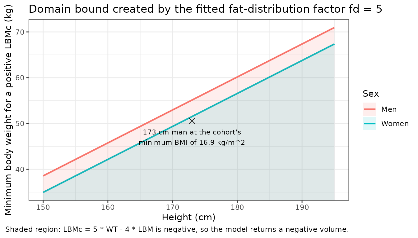

Virtual cohort

Individual patient data are not public. The cohort below approximates the Table 1 demographics of hospital A – 29% women, median BMI 24.6 kg/m^2 (range 16.9-35.3), sex-appropriate heights – and is then restricted to the positive-LBMc domain above. The number of draws that restriction removes is reported rather than silently absorbed.

# set.seed() seeds R's RNG, which is what draws the covariates below, so the
# COHORT is reproducible. It does NOT seed rxode2's eta sampler, whose streams
# are partitioned per solver thread -- so every assertion on an eta-driven
# quantity downstream is written to hold for any draw.
set.seed(20190201)

n_per_arm <- 200L

draw_subjects <- function(n_draw) {
  sexf <- rbinom(n_draw, 1L, 0.29)
  ht <- round(ifelse(sexf == 1L, rnorm(n_draw, 163, 6.5), rnorm(n_draw, 176, 7)))
  ht <- pmin(pmax(ht, 150), 193) # Table 1 height range
  bmi <- pmin(pmax(rnorm(n_draw, 24.6, 3.6), 16.9), 35.3) # Table 1 BMI range
  tibble::tibble(
    SEXF = sexf, HT = ht,
    WT = round(pmin(pmax(bmi * (ht / 100)^2, 40), 123), 1), # Table 1 weight range
    # CKD-EPI eGFR; enters only through fr, which the final model fixes at 0.
    CRCL = round(pmin(pmax(rnorm(n_draw, 95, 22), 25), 150), 1)
  ) |>
    dplyr::mutate(
      LBM = ifelse(SEXF == 1L, 45.5, 50.0) + 0.9 * (HT - 152),
      in_domain = WT > 0.8 * LBM
    )
}

pool <- draw_subjects(3000L)
n_dropped <- sum(!pool$in_domain)
cat(sprintf(
  "domain restriction: %d of %d draws (%.1f%%) had WT <= 0.8 * LBM and were dropped\n",
  n_dropped, nrow(pool), 100 * n_dropped / nrow(pool)
))
#> domain restriction: 106 of 3000 draws (3.5%) had WT <= 0.8 * LBM and were dropped
stopifnot(n_dropped > 0) # the restriction is doing work, not decorative

subjects <- pool |>
  dplyr::filter(in_domain) |>
  head(2L * n_per_arm) |>
  dplyr::mutate(id = seq_len(dplyr::n())) |>
  dplyr::select(id, SEXF, HT, WT, CRCL, LBM)

stopifnot(nrow(subjects) == 2L * n_per_arm)

# 40 days of dosing, not the 14 that a median half-life of ~13 h would suggest.
# The 122% CV on Vd puts individual half-lives as high as ~480 h, and a subject
# who has not accumulated to steady state has an AUC over the final interval
# well below F * Dose / CL -- measured at 14 days, 10% of a 100-subject draw
# failed the identity, down to 38% recovery. Dose events are cheap; only
# observation rows cost, and those are confined to the first and last intervals.
regimens <- tibble::tribble(
  ~regimen,             ~amt, ~ii, ~n_dose,
  "600/100 mg q12h",     600,  12,     80L,
  "800/100 mg q24h",     800,  24,     40L
)

t_end <- 960 # h = 40 days; identical for both arms

make_arm <- function(reg, subj) {
  last_dose <- reg$ii * (reg$n_dose - 1L)
  obs_times <- sort(unique(c(
    seq(0, 24, by = 0.5), # first dosing interval, for the accumulation view
    last_dose, # exact interval start
    # Log-spaced immediately after the dose so the sharp early peak of a
    # low-volume subject is resolved, then uniform across the interval.
    last_dose + exp(seq(log(0.01), log(reg$ii), length.out = 120)),
    seq(last_dose, t_end, length.out = 97) # includes BOTH endpoints exactly,
  ))) # which cmin needs
  dplyr::bind_rows(
    subj |>
      tidyr::crossing(time = reg$ii * seq(0L, reg$n_dose - 1L)) |>
      dplyr::mutate(amt = reg$amt, evid = 1L, cmt = "depot"),
    subj |>
      tidyr::crossing(time = obs_times) |>
      dplyr::mutate(amt = NA_real_, evid = 0L, cmt = "central")
  ) |>
    dplyr::mutate(regimen = reg$regimen, ii_h = reg$ii, last_dose = last_dose)
}

events <- dplyr::bind_rows(
  make_arm(regimens[1, ], subjects[1:n_per_arm, ]),
  make_arm(regimens[2, ], subjects[(n_per_arm + 1):(2 * n_per_arm), ])
) |>
  dplyr::arrange(id, time, evid)

# IDs are disjoint across arms, so no subject can silently receive both.
stopifnot(
  !anyDuplicated(unique(events[, c("id", "time", "evid")])),
  length(intersect(
    unique(events$id[events$regimen == regimens$regimen[1]]),
    unique(events$id[events$regimen == regimens$regimen[2]])
  )) == 0L,
  all(subjects$WT > 0.8 * subjects$LBM),
  all(subjects$LBM + (subjects$WT - subjects$LBM) * 5 > 0)
)

Simulation

sim <- rxode2::rxSolve(
  ui, events,
  omega = ui$omega, # mandatory: see the note in the cohort chunk
  keep = c("regimen", "WT", "HT", "SEXF", "CRCL", "ii_h", "last_dose"),
  returnType = "data.frame"
)

stopifnot(
  all(c("depot", "central") %in% names(sim)),
  # the population solve really did sample IIV (the reverse of the omega trap)
  dplyr::n_distinct(round(sim$vd, 8)) > 100L,
  dplyr::n_distinct(round(sim$cl_nonren, 8)) > 100L,
  # and the drawn volumes stayed positive over the restricted cohort
  all(sim$vc > 0), all(sim$cl > 0), !anyNA(sim$Cc)
)

The cohort’s realised variability is a draw, so the check below is deliberately loose: it confirms the omega^2 = log(1 + CV^2) encoding put the right order of magnitude of spread on each parameter, not that any particular draw reproduced the published SD.

iiv <- sim |>
  dplyr::distinct(id, cl_nonren, vd) |>
  dplyr::summarise(
    `CLm median (L/h/70 kg)` = median(cl_nonren),
    `CLm CV (%)` = 100 * sd(cl_nonren) / mean(cl_nonren),
    `Vd median (L/kg LBMc)` = median(vd),
    `Vd CV (%)` = 100 * sd(vd) / mean(vd)
  )

# Published: CLm 9.47 with SD 6.19 (CV 65.4 %); Vd 2.13 with SD 2.60 (CV 122.1 %).
# The MEDIAN of a log-normal whose median is the published mean is the published
# mean, so those are checked with generous multiplicative bounds; the CVs are
# checked only for order of magnitude because a 400-subject draw of a CV-122 %
# log-normal has a very wide sampling distribution.
stopifnot(
  iiv$`CLm median (L/h/70 kg)` > 9.47 / 1.5, iiv$`CLm median (L/h/70 kg)` < 9.47 * 1.5,
  iiv$`Vd median (L/kg LBMc)` > 2.13 / 1.5, iiv$`Vd median (L/kg LBMc)` < 2.13 * 1.5,
  iiv$`CLm CV (%)` > 35, iiv$`CLm CV (%)` < 110,
  iiv$`Vd CV (%)` > 60, iiv$`Vd CV (%)` < 220
)

iiv |>
  dplyr::mutate(dplyr::across(dplyr::everything(), \(x) round(x, 2))) |>
  knitr::kable(caption = "Realised cohort variability against the published CLm 9.47 (SD 6.19) and Vd 2.13 (SD 2.60).")

Realised cohort variability against the published CLm 9.47 (SD 6.19) and Vd 2.13 (SD 2.60).
CLm median (L/h/70 kg)	CLm CV (%)	Vd median (L/kg LBMc)	Vd CV (%)
10.01	59	2.01	139.62

Simulated concentration-time behaviour

The paper publishes no concentration-versus-time figure – its Figures 1 and 2 are Passing-Bablok and Bland-Altman agreement plots built from individual patient records, which are not public. The panels below therefore characterise the packaged model rather than replicating a published figure.

sim |>
  dplyr::filter(!is.na(Cc), time <= 24) |>
  dplyr::group_by(regimen, time) |>
  dplyr::summarise(
    Q05 = quantile(Cc, 0.05), Q50 = quantile(Cc, 0.50), Q95 = quantile(Cc, 0.95),
    .groups = "drop"
  ) |>
  ggplot(aes(time, Q50)) +
  geom_ribbon(aes(ymin = Q05, ymax = Q95), alpha = 0.25, fill = "steelblue") +
  geom_line(linewidth = 0.8) +
  facet_wrap(~regimen) +
  scale_x_continuous(breaks = seq(0, 24, 6)) +
  labs(
    x = "Time after first dose (h)", y = "Darunavir concentration (mg/L)",
    title = "First 24 h after treatment start",
    caption = "Median with 5th-95th percentile band, 200 virtual patients per regimen."
  ) +
  theme_bw()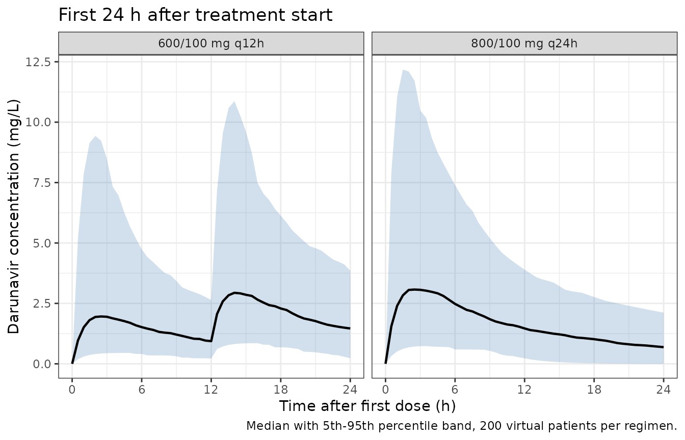

sim |>
  dplyr::filter(!is.na(Cc), time >= last_dose) |>
  dplyr::mutate(tad = time - last_dose) |>
  dplyr::group_by(regimen, tad) |>
  dplyr::summarise(
    Q05 = quantile(Cc, 0.05), Q50 = quantile(Cc, 0.50), Q95 = quantile(Cc, 0.95),
    .groups = "drop"
  ) |>
  ggplot(aes(tad, Q50)) +
  geom_ribbon(aes(ymin = Q05, ymax = Q95), alpha = 0.25, fill = "darkorange") +
  geom_line(linewidth = 0.8) +
  geom_hline(
    data = tibble::tibble(
      regimen = regimens$regimen, cutoff = c(2.60, 1.07)
    ),
    aes(yintercept = cutoff), linetype = "dashed"
  ) +
  facet_wrap(~regimen, scales = "free_x") +
  labs(
    x = "Time after the last dose (h)", y = "Darunavir concentration (mg/L)",
    title = "Steady state, final dosing interval",
    caption = paste(
      "Median with 5th-95th percentile band. Dashed line: the follow-up trough",
      "cut-off quoted in the Discussion (1.07 mg/L once daily, 2.60 mg/L twice daily)."
    )
  ) +
  theme_bw()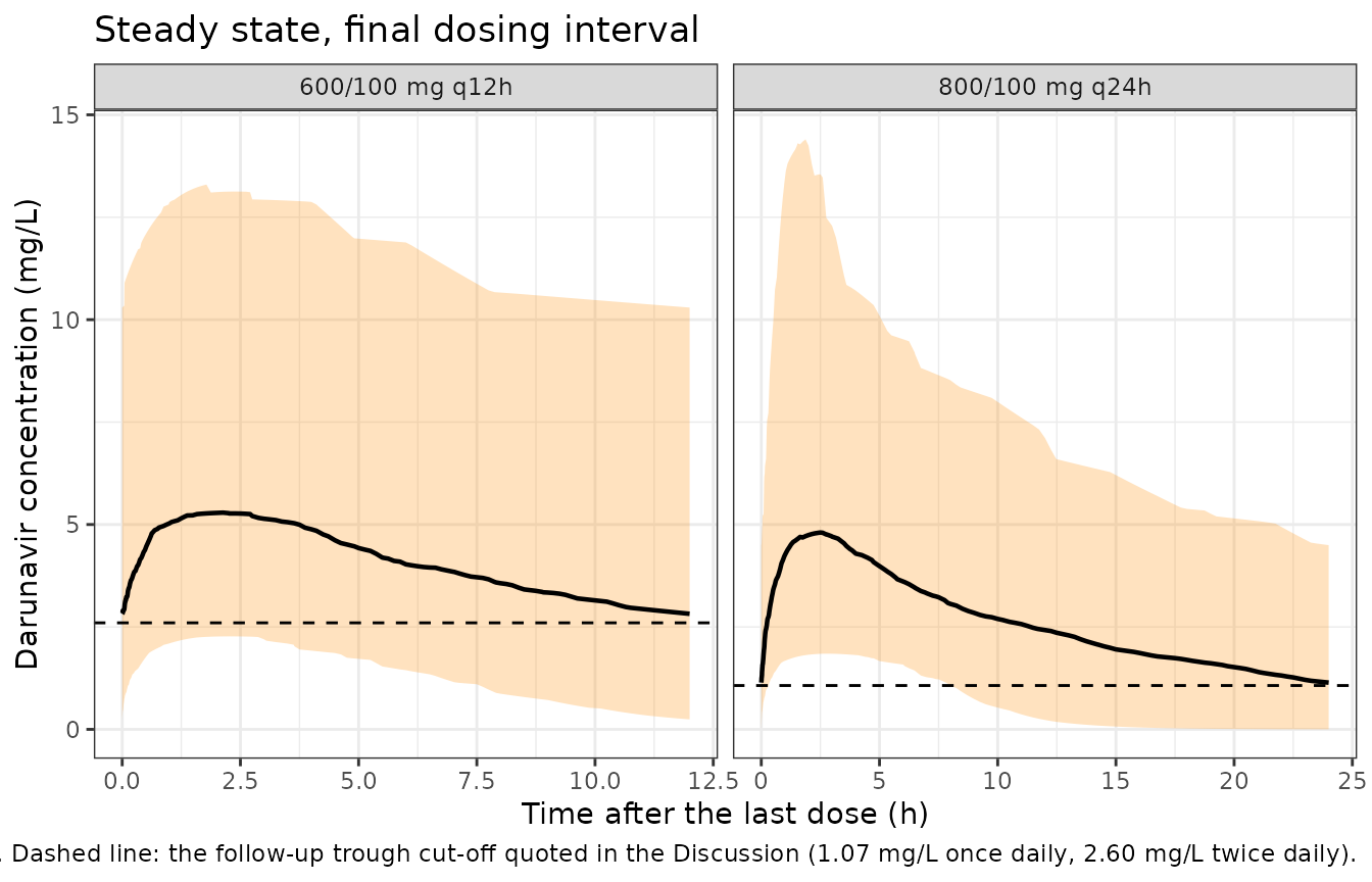

PKNCA validation

Steady-state NCA over the final dosing interval of each regimen, per PKNCA recipe 3. The observation grid places records at both interval endpoints exactly, which cmin needs.

Note the regimen column on the intervals frame. Without it PKNCA applies every interval row to every group, so each subject would receive results for both the q12h and the q24h window; pivot_wider() then silently produces list columns and an anyNA() check on them returns FALSE regardless of content – a gate that cannot go red. The type assertions below exist for that reason.

sim_nca <- sim |>
  dplyr::filter(!is.na(Cc)) |>
  dplyr::transmute(id, time, Cc, regimen = as.character(regimen))

# Guarantee a time = 0 record per subject; for extravascular dosing the
# pre-dose concentration is 0.
sim_nca <- dplyr::bind_rows(
  sim_nca,
  sim_nca |> dplyr::distinct(id, regimen) |> dplyr::mutate(time = 0, Cc = 0)
) |>
  dplyr::distinct(id, regimen, time, .keep_all = TRUE) |>
  dplyr::arrange(id, time)

dose_df <- events |>
  dplyr::filter(evid == 1L) |>
  dplyr::select(id, time, amt, regimen) |>
  dplyr::mutate(regimen = as.character(regimen))

conc_obj <- PKNCA::PKNCAconc(
  as.data.frame(sim_nca), Cc ~ time | regimen + id,
  concu = "mg/L", timeu = "h"
)
dose_obj <- PKNCA::PKNCAdose(
  as.data.frame(dose_df), amt ~ time | regimen + id,
  doseu = "mg", route = "extravascular"
)

ss_windows <- events |>
  dplyr::distinct(regimen, ii_h, last_dose) |>
  dplyr::arrange(regimen) # PKNCA orders groups alphabetically

intervals <- data.frame(
  regimen = as.character(ss_windows$regimen), # binds each window to its own arm
  start = ss_windows$last_dose,
  end = ss_windows$last_dose + ss_windows$ii_h,
  cmax = TRUE, tmax = TRUE, cmin = TRUE,
  auclast = TRUE, cav = TRUE,
  stringsAsFactors = FALSE
)

nca_res <- PKNCA::pk.nca(PKNCA::PKNCAdata(conc_obj, dose_obj, intervals = intervals))

nca_par <- c("cmax", "tmax", "cmin", "auclast", "cav")
nca_raw <- as.data.frame(nca_res$result) |>
  dplyr::filter(PPTESTCD %in% nca_par)

# One result per subject per parameter -- proves the interval grouping worked
# and that the pivot below cannot produce a list column.
stopifnot(
  nrow(dplyr::count(nca_raw, regimen, id, PPTESTCD) |> dplyr::filter(n > 1L)) == 0L
)

nca_tbl <- nca_raw |>
  dplyr::select(regimen, id, PPTESTCD, PPORRES) |>
  tidyr::pivot_wider(names_from = PPTESTCD, values_from = PPORRES)

stopifnot(
  nrow(nca_tbl) == 2L * n_per_arm, # every subject produced a result
  # Type guard: a list column would make every anyNA() below pass vacuously.
  all(vapply(nca_tbl[nca_par], is.numeric, logical(1))),
  !anyNA(nca_tbl$auclast), !anyNA(nca_tbl$cmin), !anyNA(nca_tbl$cmax)
)

At steady state a linear model must satisfy CL * AUC(0-tau) = F * Dose, evaluated per subject against that subject’s own drawn clearance. It is exact up to quadrature, so it is a structural gate rather than a statistical one, and it is the check that would catch a lost dose event, a wrong f(depot) target or a mis-scaled interval.

The identity only holds once a subject has actually accumulated to steady state, which is not automatic here: the 122% CV on Vd gives some subjects half-lives of several hundred hours. Each subject’s attainment is therefore tested explicitly against its own half-life and the shortfall is reported rather than absorbed into a loosened tolerance.

subject_pk <- sim |>
  dplyr::distinct(id, regimen, cl, vc) |>
  dplyr::mutate(
    regimen = as.character(regimen),
    thalf = log(2) * vc / cl,
    # 7 half-lives leaves under 1% of the approach to steady state outstanding.
    ss_attained = t_end >= 7 * thalf
  )
stopifnot(nrow(subject_pk) == 2L * n_per_arm) # one row per subject, no fan-out

mb <- nca_tbl |>
  dplyr::left_join(subject_pk, by = c("id", "regimen")) |>
  dplyr::left_join(regimens |> dplyr::select(regimen, dose_amt = amt), by = "regimen") |>
  dplyr::mutate(recovered = cl * auclast / (0.82 * dose_amt))

stopifnot(nrow(mb) == 2L * n_per_arm, !anyNA(mb$recovered), !anyNA(mb$ss_attained))

n_not_ss <- sum(!mb$ss_attained)
cat(sprintf(
  paste0(
    "half-life: median %.1f h, max %.1f h\n",
    "not yet at steady state after %d h (t1/2 > %.0f h): %d of %d subjects\n",
    "CL * AUCtau / (F * Dose), steady-state subjects only: %.4f - %.4f\n"
  ),
  median(mb$thalf), max(mb$thalf), t_end, t_end / 7, n_not_ss, nrow(mb),
  min(mb$recovered[mb$ss_attained]), max(mb$recovered[mb$ss_attained])
))
#> half-life: median 12.9 h, max 748.0 h
#> not yet at steady state after 960 h (t1/2 > 137 h): 7 of 400 subjects
#> CL * AUCtau / (F * Dose), steady-state subjects only: 0.9944 - 1.0000

stopifnot(
  # The gate must have most of the cohort to test.
  sum(mb$ss_attained) > 0.9 * nrow(mb),
  # Quadrature over one interval plus the < 1% of accumulation still outstanding
  # at 7 half-lives. Observed maxima across draws sat at or under 1.0%; 3%
  # leaves headroom for which subjects land near the attainment boundary while
  # still going red on a structural break (dropping f(depot) moves this 22%).
  max(abs(mb$recovered[mb$ss_attained] - 1)) < 0.03
)

The same identity on the deterministic typical-value covariate grid, where every subject is comfortably at steady state, is where the tight bound belongs.

ss_typ <- lapply(seq_len(nrow(regimens)), function(i) {
  reg <- regimens[i, ]
  ld <- reg$ii * (reg$n_dose - 1L)
  ev <- dplyr::bind_rows(
    cov_grid |> tidyr::crossing(time = reg$ii * seq(0L, reg$n_dose - 1L)) |>
      dplyr::mutate(amt = reg$amt, evid = 1L, cmt = "depot"),
    cov_grid |> tidyr::crossing(time = sort(unique(c(
      ld, ld + exp(seq(log(0.01), log(reg$ii), length.out = 150)),
      seq(ld, ld + reg$ii, length.out = 97)
    )))) |>
      dplyr::mutate(amt = NA_real_, evid = 0L, cmt = "central")
  ) |>
    dplyr::arrange(id, time, evid)
  s <- rxode2::rxSolve(typ, ev, omega = NA, returnType = "data.frame")
  s <- s[!is.na(s$Cc) & s$time >= ld, ]
  # pk.calc.auc.last() defaults its interval to start at 0, so it returns NA on
  # an absolute-time window starting at 936 h. Pass time after the dose instead.
  s$tad <- s$time - ld
  s |>
    dplyr::group_by(id) |>
    dplyr::summarise(
      cl = dplyr::first(cl),
      auctau = PKNCA::pk.calc.auc.last(conc = Cc, time = tad),
      .groups = "drop"
    ) |>
    dplyr::mutate(regimen = reg$regimen, recovered = cl * auctau / (0.82 * reg$amt))
}) |>
  dplyr::bind_rows()
#> Warning: multi-subject simulation without without 'omega'
#> Warning: multi-subject simulation without without 'omega'

stopifnot(
  nrow(ss_typ) == 2L * nrow(cov_grid),
  !anyNA(ss_typ$recovered),
  # Deterministic: quadrature only. Realised maximum deviation 0.03%.
  max(abs(ss_typ$recovered - 1)) < 0.005
)
cat(sprintf(
  "typical-value steady-state recovery: %.5f - %.5f over %d covariate/regimen combinations\n",
  min(ss_typ$recovered), max(ss_typ$recovered), nrow(ss_typ)
))
#> typical-value steady-state recovery: 0.99995 - 0.99999 over 24 covariate/regimen combinations

nca_summary <- nca_tbl |>
  dplyr::group_by(regimen) |>
  dplyr::summarise(
    n = dplyr::n(),
    cmax = median(cmax), tmax = median(tmax),
    cmin = median(cmin), cav = median(cav), auclast = median(auclast),
    cmin_p05 = quantile(cmin, 0.05), cmin_p95 = quantile(cmin, 0.95),
    .groups = "drop"
  )

nca_summary |>
  dplyr::transmute(
    regimen, n,
    cmax = round(cmax, 2), tmax = round(tmax, 2),
    cmin = round(cmin, 2),
    cmin_range = sprintf("%.2f - %.2f", cmin_p05, cmin_p95),
    cav = round(cav, 2), auclast = round(auclast, 1)
  ) |>
  dplyr::rename(
    "Regimen" = regimen, "N" = n,
    "Cmax,ss (mg/L)" = cmax, "Tmax,ss (h)" = tmax,
    "Ctrough,ss (mg/L)" = cmin, "Ctrough 5th-95th pctile" = cmin_range,
    "Cavg,ss (mg/L)" = cav, "AUC0-tau,ss (mg*h/L)" = auclast
  ) |>
  knitr::kable(caption = "Median steady-state NCA parameters by regimen (PKNCA, final dosing interval after 40 days, 200 virtual patients per arm). Ctrough,ss is PKNCA's cmin over the interval.")

Median steady-state NCA parameters by regimen (PKNCA, final dosing interval after 40 days, 200 virtual patients per arm). Ctrough,ss is PKNCA’s cmin over the interval.
Regimen	N	Cmax,ss (mg/L)	Tmax,ss (h)	Ctrough,ss (mg/L)	Ctrough 5th-95th pctile	Cavg,ss (mg/L)	AUC0-tau,ss (mg*h/L)
600/100 mg q12h	200	5.33	2.26	2.82	2.82 - 2.82	4.23	50.8
800/100 mg q24h	200	4.87	2.60	1.14	1.14 - 1.14	2.64	63.4

Comparison against published NCA

The source paper reports no NCA parameters. Table 2 holds only model parameters; there is no Cmax, Tmax, AUC or half-life anywhere in the paper or its four supplements, and the published validation is the agreement analysis described above. nlmixr2lib::ncaComparisonTable() is therefore not used here, because there is no reference column to put beside the simulated one.

The only exposure numbers the paper does print are the two trough cut-offs the Groningen protocol uses to trigger TDM follow-up: 1.07 mg/L for once-daily and 2.60 mg/L for twice-daily dosing (Discussion). These are decision thresholds taken from the local protocol, not model outputs and not population predictions, so they are recorded below as orientation rather than gated: an adherent typical patient is expected to sit above them, which is the direction the model gives.

typical_ss <- function() {
  # One typical patient per regimen at the Table 1 median covariates, no IIV.
  med <- tibble::tibble(SEXF = 0, HT = 173, WT = 72, CRCL = 95)
  out <- lapply(seq_len(nrow(regimens)), function(i) {
    reg <- regimens[i, ]
    last_dose <- reg$ii * (reg$n_dose - 1L)
    ev <- dplyr::bind_rows(
      med |> tidyr::crossing(time = reg$ii * seq(0L, reg$n_dose - 1L)) |>
        dplyr::mutate(id = 1L, amt = reg$amt, evid = 1L, cmt = "depot"),
      med |> tidyr::crossing(time = seq(last_dose, last_dose + reg$ii, length.out = 97)) |>
        dplyr::mutate(id = 1L, amt = NA_real_, evid = 0L, cmt = "central")
    ) |>
      dplyr::arrange(time, evid)
    s <- rxode2::rxSolve(typ, ev, omega = NA, returnType = "data.frame")
    s <- s[!is.na(s$Cc), ]
    tibble::tibble(
      regimen = reg$regimen, cmax = max(s$Cc), ctrough = min(s$Cc),
      cutoff = if (reg$ii == 24) 1.07 else 2.60
    )
  })
  dplyr::bind_rows(out)
}
typ_ss <- typical_ss()

typ_ss |>
  dplyr::transmute(
    regimen,
    `Typical Cmax,ss (mg/L)` = round(cmax, 2),
    `Typical Ctrough,ss (mg/L)` = round(ctrough, 2),
    `Protocol follow-up cut-off (mg/L)` = cutoff,
    `Above cut-off` = ctrough > cutoff
  ) |>
  dplyr::rename("Regimen" = regimen) |>
  knitr::kable(caption = "Typical-value steady-state troughs at the Table 1 median male covariates, beside the follow-up cut-offs quoted in the Discussion. Orientation only -- the cut-offs are protocol decision thresholds, not published model predictions.")

Typical-value steady-state troughs at the Table 1 median male covariates, beside the follow-up cut-offs quoted in the Discussion. Orientation only – the cut-offs are protocol decision thresholds, not published model predictions.
Regimen	Typical Cmax,ss (mg/L)	Typical Ctrough,ss (mg/L)	Protocol follow-up cut-off (mg/L)	Above cut-off
600/100 mg q12h	5.07	3.15	2.60	TRUE
800/100 mg q24h	4.34	1.44	1.07	TRUE


# Gated only on being physically sensible and above the 0.2 mg/L assay LLOQ:
# this is a deterministic typical-value quantity, so the bound is tight.
stopifnot(
  all(typ_ss$ctrough > 0.2), # the paper's lower limit of quantification
  all(typ_ss$cmax > typ_ss$ctrough),
  all(typ_ss$cmax < 20) # a mis-scaled volume or dose would blow this
)

Assumptions and deviations

Interpretation of the reported “Mean (SD)” pairs

MWPharm’s KinPop reports each population parameter as a mean with a separate interindividual SD in the parameter’s own units (Table 2; Supplement 1 and Supplement 3 print the same value (SD) shape), while the Methods state that “pharmacokinetic parameters were assumed to be log-normally distributed”. The packaged model follows this library’s standing convention for that combination: the printed mean is carried as the typical value and the printed SD is converted to a log-scale variance by omega^2 = log(1 + CV^2) with CV = SD / mean, giving 0.355749 for CLm (CV 65.4%) and 0.912284 for Vd (CV 122.1%).

The alternative reading is that the printed mean is the arithmetic mean of the log-normal, in which case the median would be mean / sqrt(1 + CV^2) – 7.93 rather than 9.47 L/h/70 kg for CLm, and 1.35 rather than 2.13 L/kg LBMc for Vd. The paper does not say which it is, and MWPharm’s convention is not documented in it. Two observations in each direction, recorded so a reader can judge:

for the arithmetic-mean reading: it makes Models 1 and 2 of Table 2 agree on a median CLm (7.63 vs 7.93 L/h/70 kg) where the median reading has them 18% apart, and it puts the implied median Vd (1.35) within 5% of the Arab-Alameddine literature prior of 1.42 L/kg LBMc that Supplement 1 carries.
for the convention used here: it is what the rest of this library does with a printed mean, it keeps the packaged typical values byte-identical to Table 2 so the source trace is checkable by eye, and it gives a typical terminal half-life of 12.8 h, closer to darunavir’s reported value than the 10.5 h the alternative gives.

A user who wants the other reading can divide each typical value by sqrt(1 + CV^2) without touching the variances.

The `fd = 5` domain bound

Documented at length in its own section above, and repeated here because it is the deviation most likely to bite. fd = 5 extrapolates the lean-body-mass correction past total body weight, so LBMc = 5 * WT - 4 * LBM and the volume of distribution is negative for any subject with WT <= 0.8 * LBM. That region is reachable inside the covariate ranges the paper itself reports for its own cohort. This is a property of the published model, not of the transcription; the virtual cohort here is restricted to the positive-LBMc region and the number of draws that restriction removed is printed.

A related point: the Methods sentence “V1 is the volume of distribution (in liters per 70 kg LBMc)” is inconsistent with Table 2’s own unit label L/kgLBMc, with the parallel sentence describing V2 as “in liters per kg LBMc”, and with dimensional sense – the per-70-kg reading would give a typical volume of 2.6 L. The per-kg reading of Table 2 is used.

`fr = 0` makes the `CRCL` column inert

The published clearance equation is CL = CLm * (WT / 70) + fr * CLcr, and fr is fixed at 0 in the final model, so creatinine clearance has no effect on any prediction. The arm is nevertheless retained in the model file, with fr encoded as e_crcl_cl_renal <- fixed(0), because Supplement 4 shows it was tested at the SPC value of 0.12 and rejected on AIC (1611.08 vs 1584.89) rather than never considered. A user can restore it by overriding e_crcl_cl_renal; the mutation control above verifies that doing so changes clearance by exactly fr * CLcr. The consequence for simulation is that a CRCL column must be supplied even though it does nothing.

CKD-EPI needs age and sex as well as serum creatinine, and the paper does not state whether a race coefficient was applied, so a user deriving the column from raw creatinine will have to choose a CKD-EPI variant.

Other assumptions

Race and ethnicity are not reported in Table 1 and are not covariates, so the virtual cohort does not model them.
Height and weight distributions. Table 1 gives medians and ranges but no SDs or joint distribution. The cohort samples sex-appropriate heights and a BMI centred on the reported median of 24.6 kg/m^2, then derives weight, so that height and weight stay physiologically paired – which matters here because the fd = 5 bound is a joint constraint on the two.
Covariates held constant. The source treats weight and serum creatinine as “continuously changing covariates” (Discussion) – that flexibility is the reason the authors chose ITSB over mixed-effects modelling. The cohort here holds them fixed per subject, which is the right choice for a steady-state exposure illustration but does not exercise the time-varying path.
Residual error combination. The assay SD is reported as the linear sum 0.2 + 0.05 * C, which is nlmixr2’s combined1() form rather than the default quadrature combination of add() and prop(). Both terms are fixed, because they describe the assay rather than a fitted quantity.
Only the final model is packaged. Table 2’s Model 1 (AIC 945.31, CLm Bayesian only) is a rejected development submodel: its volume was held at the literature value, which “implies that the volume of distribution … is the same for each patient, which does not seem logical” (Results), and its external validation was markedly worse (r^2 = 0.85 against 0.97; 92.3% of predictions within the limits of agreement against 98.2%). Per the base-versus-final policy the library packages the final model only. The two-compartment model explored in Supplement 3 is likewise not packaged; the paper rejected it.
No published NCA and no reproducible published figure. Discussed in the PKNCA section. Every numeric gate in this vignette is therefore either an algebraic identity of the published equations or a mutation control on one of them, not a comparison against a published exposure number – because the paper contains none.
Ka is not identifiable in these data. It is fixed at the Arab-Alameddine literature value of 1.04 1/h because “the low number of darunavir samples drawn in the absorption phase; 0-4 hours after drug intake” made estimation impossible (Discussion). Simulated Tmax and the shape of the absorption phase are therefore inherited from that external source, not fitted here, and should not be treated as validated by this paper.
Unmodelled mechanisms the authors name. Food intake, pharmacogenomics and binding to alpha-1-acid glycoprotein are all absent from the model and are listed in the Discussion as candidate explanations for the residual overestimation at low concentrations. Ritonavir is present in every regimen as a fixed-dose booster and is not modelled as a covariate, so the packaged model describes boosted darunavir only.

sessionInfo()
#> R version 4.6.1 (2026-06-24)
#> Platform: x86_64-pc-linux-gnu
#> Running under: Ubuntu 24.04.5 LTS
#> 
#> Matrix products: default
#> BLAS:   /usr/lib/x86_64-linux-gnu/openblas-pthread/libblas.so.3 
#> LAPACK: /usr/lib/x86_64-linux-gnu/openblas-pthread/libopenblasp-r0.3.26.so;  LAPACK version 3.12.0
#> 
#> locale:
#>  [1] LC_CTYPE=C.UTF-8       LC_NUMERIC=C           LC_TIME=C.UTF-8       
#>  [4] LC_COLLATE=C.UTF-8     LC_MONETARY=C.UTF-8    LC_MESSAGES=C.UTF-8   
#>  [7] LC_PAPER=C.UTF-8       LC_NAME=C              LC_ADDRESS=C          
#> [10] LC_TELEPHONE=C         LC_MEASUREMENT=C.UTF-8 LC_IDENTIFICATION=C   
#> 
#> time zone: UTC
#> tzcode source: system (glibc)
#> 
#> attached base packages:
#> [1] stats     graphics  grDevices utils     datasets  methods   base     
#> 
#> other attached packages:
#> [1] ggplot2_4.0.3         tidyr_1.3.2           dplyr_1.2.1          
#> [4] rxode2_5.1.8          PKNCA_0.12.1          nlmixr2lib_0.3.2.9000
#> 
#> loaded via a namespace (and not attached):
#>  [1] gtable_0.3.6        xfun_0.61           bslib_0.12.0       
#>  [4] rxode2lincmt_0.1.0  lattice_0.22-9      vctrs_0.7.3        
#>  [7] tools_4.6.1         generics_0.1.4      parallel_4.6.1     
#> [10] tibble_3.3.1        symengine_0.2.13    pkgconfig_2.0.3    
#> [13] data.table_1.18.6.1 checkmate_2.3.4     RColorBrewer_1.1-3 
#> [16] S7_0.2.2            desc_1.4.3          lifecycle_1.0.5    
#> [19] compiler_4.6.1      farver_2.1.2        textshaping_1.0.5  
#> [22] fontawesome_0.5.3   htmltools_0.5.9     sys_3.4.3          
#> [25] sass_0.4.10         yaml_2.3.12         pillar_1.11.1      
#> [28] pkgdown_2.2.1       crayon_1.5.3        jquerylib_0.1.4    
#> [31] whisker_0.4.1       openssl_2.4.2       cachem_1.1.0       
#> [34] nlme_3.1-169        tidyselect_1.2.1    digest_0.6.39      
#> [37] lotri_1.0.5         purrr_1.2.2         labeling_0.4.3     
#> [40] rxode2ll_2.0.18     fastmap_1.2.0       grid_4.6.1         
#> [43] cli_3.6.6           dparser_1.3.1-13    magrittr_2.0.5     
#> [46] withr_3.0.3         scales_1.4.0        backports_1.5.1    
#> [49] rmarkdown_2.32      otel_0.2.0          askpass_1.2.1      
#> [52] ragg_1.5.2          memoise_2.0.1       evaluate_1.0.5     
#> [55] knitr_1.52          rex_1.2.2           PreciseSums_0.7    
#> [58] rlang_1.3.0         downlit_0.4.5       Rcpp_1.1.2         
#> [61] glue_1.8.1          xml2_1.6.0          jsonlite_2.0.0     
#> [64] R6_2.6.1            systemfonts_1.3.2   fs_2.1.0

Model and source

Population

Source trace

Structural verification

The solved system keeps both compartments

Every derived covariate term matches the published equations

The solved profile matches its own closed form

Mutation controls – each fixed switch is live, not dead code

Dose recovery through PKNCA

The fd = 5 domain bound

Virtual cohort

Simulation

Simulated concentration-time behaviour

PKNCA validation

Comparison against published NCA

Assumptions and deviations

Interpretation of the reported “Mean (SD)” pairs

The fd = 5 domain bound

fr = 0 makes the CRCL column inert

Other assumptions

The `fd = 5` domain bound

The `fd = 5` domain bound

`fr = 0` makes the `CRCL` column inert