Paracetamol (Anderson 1998)
Source:vignettes/articles/Anderson_1998_paracetamol.Rmd
Anderson_1998_paracetamol.RmdModel and source
- Citation: Anderson BJ, Holford NHG, Woollard GA, Chan PLS (1998). Paracetamol plasma and cerebrospinal fluid pharmacokinetics in children. British Journal of Clinical Pharmacology 46(3):237-243. doi:10.1046/j.1365-2125.1998.00780.x.
- Description: One-compartment oral PK model for paracetamol (acetaminophen) with an explicit cerebrospinal-fluid (CSF) equilibration compartment in nine ventilator-dependent children (5 months to 12 years) with indwelling ventricular drains for raised intracranial pressure (Anderson 1998 NONMEM fit, Table 3). First-order absorption, single nasogastric dose of 40 mg/kg paracetamol elixir, plasma + CSF sampled hourly for 4 h and 2-hourly through 10 h. CSF concentration follows the plasma concentration with first-order equilibration rate keq = ln(2)/teq and steady-state ratio PC = Ccsf/Cc. Parameters are standardized to a 70 kg adult using fixed allometric exponents (0.75 on CL, 1 on V, 0.25 on the equilibration half-time teq; keq therefore scales with exponent -0.25). The published equation 2 for residual error var = SF^2 * (C^PWR + V) is unconventional and the NONMEM PWR and V terms are not reported; placeholder additive residual SDs are used so the model simulates plausibly (see vignette Errata).
- Article: https://doi.org/10.1046/j.1365-2125.1998.00780.x
Population
Anderson 1998 reports a single-centre paediatric intensive-care study at Auckland Children’s Hospital, New Zealand. Nine ventilator-dependent children (3 female, 6 male) aged 5 months to 12 years (median 5 years) and weighing 8 to 50 kg (median 20 kg) received a single nasogastric dose of paracetamol elixir 40 mg/kg via an enteral feeding tube. All children had external ventricular drains placed for raised intracranial pressure (>20 mmHg); arterial blood and CSF were sampled hourly for the first 4 h and 2-hourly through 10 h. Patient 1 was studied on two separate occasions five days apart (Tables 1-3 of the source). Children with CSF red-blood-cell counts above 4 x 10^10 /L were excluded. Diagnoses spanned closed head injury, intracranial haematoma, encephalitis, posterior fossa tumour, and a Dandy-Walker cyst (Table 1).
The same population metadata is available programmatically via
readModelDb("Anderson_1998_paracetamol")$population.
Source trace
Per-parameter provenance is recorded as inline ini()
comments in
inst/modeldb/specificDrugs/Anderson_1998_paracetamol.R. The
table below collects them in one place.
| Equation / parameter | Value (NONMEM final) | Source location |
|---|---|---|
lka |
0.77 /h | Anderson 1998 Table 3, geometric mean |
lcl |
10.2 L/h | Anderson 1998 Table 3, geometric mean |
lvc |
67.1 L | Anderson 1998 Table 3, geometric mean |
lkeq = ln(2)/teq |
0.963 /h (teq=0.72h) | Anderson 1998 Table 3, geometric mean |
lpc |
1.18 | Anderson 1998 Table 3, geometric mean |
allo_cl (fixed) |
0.75 | Anderson 1998 Methods, allometric paragraph |
allo_vc (fixed) |
1 | Anderson 1998 Methods, allometric paragraph |
allo_keq (fixed) |
-0.25 | Anderson 1998 Methods (teq exponent 0.25 -> keq exponent -0.25) |
| IIV ka (CV 49%) | omega^2 = 0.2153 | Anderson 1998 Table 3 %CV row |
| IIV CL (CV 47%) | omega^2 = 0.1996 | Anderson 1998 Table 3 %CV row |
| IIV V (CV 58%) | omega^2 = 0.2900 | Anderson 1998 Table 3 %CV row |
| IIV keq (CV 117%) | omega^2 = 0.8623 | Anderson 1998 Table 3 %CV row (reported on teq; CV is identical for keq) |
| IIV PC (CV 8%) | omega^2 = 0.006379 | Anderson 1998 Table 3 %CV row |
| addSd plasma (placeholder) | 1.5 mg/L | see Assumptions and deviations |
| addSd_Ccsf (placeholder) | 1.5 mg/L | see Assumptions and deviations |
| ODE system | n/a | Anderson 1998 equation 1 |
| Residual-error form | n/a | Anderson 1998 equation 2 (and Methods NONMEM paragraph) |
Virtual cohort
The original observed data are not publicly available. The cohort below approximates the Table 1 demographics: nine ventilator-dependent children with body weights matching the published per-patient weights, each receiving a single 40 mg/kg nasogastric dose.
set.seed(1998)

# Per-patient body weights from Anderson 1998 Table 1.
table1_weights_kg <- c(16, 8, 50, 30, 8, 40, 45, 14, 20)
n_subjects <- length(table1_weights_kg)

# Build the event table: one nasogastric dose at time 0 (cmt = "depot"), plus
# parallel observation rows for the two outputs Cc (plasma) and Ccsf (CSF).
obs_grid <- c(seq(0, 4, by = 0.25), seq(4.5, 10, by = 0.5))

per_subject <- tibble(
  id = seq_len(n_subjects),
  WT = table1_weights_kg,
  dose_mg = 40 * WT
)

dose_rows <- per_subject |>
  transmute(id, time = 0, amt = dose_mg, cmt = "depot",
            evid = 1L, ii = NA_real_, addl = NA_integer_, WT)

obs_cc <- per_subject |>
  tidyr::crossing(time = obs_grid) |>
  transmute(id, time, amt = NA_real_, cmt = "Cc",
            evid = 0L, ii = NA_real_, addl = NA_integer_, WT)

obs_csf <- per_subject |>
  tidyr::crossing(time = obs_grid) |>
  transmute(id, time, amt = NA_real_, cmt = "Ccsf",
            evid = 0L, ii = NA_real_, addl = NA_integer_, WT)

events <- bind_rows(dose_rows, obs_cc, obs_csf) |>
  arrange(id, time, desc(evid))

stopifnot(!anyDuplicated(unique(events[, c("id", "time", "evid", "cmt")])))
Simulation
mod <- rxode2::rxode2(readModelDb("Anderson_1998_paracetamol"))
#> ℹ parameter labels from comments will be replaced by 'label()'

# Typical-value simulation (no IIV, no residual): reproduces the population
# mean trajectory for direct comparison with Anderson 1998 Figure 2.
mod_typical <- rxode2::zeroRe(mod)
sim_typical <- rxode2::rxSolve(
  mod_typical, events = events,
  keep = c("WT"),
  returnType = "data.frame"
)
#> ℹ omega/sigma items treated as zero: 'etalka', 'etalcl', 'etalvc', 'etalkeq', 'etalpc'
#> Warning: multi-subject simulation without without 'omega'
sim_typ_cc  <- sim_typical |> filter(CMT == 4)
sim_typ_csf <- sim_typical |> filter(CMT == 5)

# Stochastic VPC: replicate the nine-patient cohort 50 times via nStud.
# Each study replicate carries fresh etas; residual error is added on top.
sim <- rxode2::rxSolve(
  mod, events = events,
  keep = c("WT"),
  returnType = "data.frame",
  nStud = 50
)
sim_cc  <- sim |> filter(CMT == 4)
sim_csf <- sim |> filter(CMT == 5)
Replicate published figures
Figure 2: Typical plasma and CSF time-concentration profiles
Anderson 1998 Figure 2 shows the plasma and CSF concentration-time profile of patient 1b (16 kg) after a single 40 mg/kg nasogastric dose, with the CSF profile lagging behind plasma by roughly one hour. The block below reproduces the typical-value profile for the same weight using the packaged model.
patient1_id <- 1
fig2 <- bind_rows(
  sim_typ_cc  |> filter(id == patient1_id) |>
    transmute(time, conc = Cc,   compartment = "Plasma (Cc)"),
  sim_typ_csf |> filter(id == patient1_id) |>
    transmute(time, conc = Ccsf, compartment = "CSF (Ccsf)")
)

ggplot(fig2, aes(time, conc, colour = compartment)) +
  geom_line(linewidth = 0.8) +
  scale_colour_manual(values = c("Plasma (Cc)" = "#1b9e77",
                                 "CSF (Ccsf)"  = "#d95f02")) +
  labs(x = "Time (h)", y = "Paracetamol concentration (mg/L)",
       colour = NULL,
       title = "Typical-value plasma and CSF profiles (16 kg child)",
       caption = "Replicates Figure 2 of Anderson 1998.")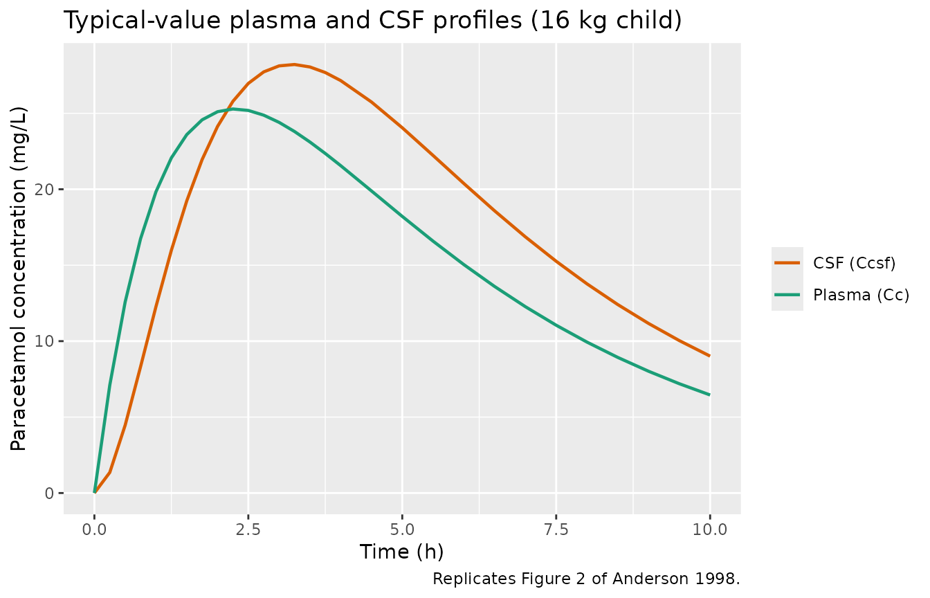
Replicates Figure 2 of Anderson 1998: typical plasma (Cc) and CSF (Ccsf) profiles for the patient-1 16 kg child receiving 40 mg/kg paracetamol elixir.
VPC by output
Stochastic simulation with the full population variability produces a spread that brackets the typical profile. The CSF percentile band shifts later and peaks lower than plasma, consistent with Figures 2-3 of the source.
make_vpc_band <- function(df, conc_col, label) {
  df |>
    group_by(time) |>
    summarise(
      Q05 = quantile(.data[[conc_col]], 0.05, na.rm = TRUE),
      Q50 = quantile(.data[[conc_col]], 0.50, na.rm = TRUE),
      Q95 = quantile(.data[[conc_col]], 0.95, na.rm = TRUE),
      .groups = "drop"
    ) |>
    mutate(compartment = label)
}

vpc <- bind_rows(
  make_vpc_band(sim_cc,  "Cc",   "Plasma (Cc)"),
  make_vpc_band(sim_csf, "Ccsf", "CSF (Ccsf)")
)

ggplot(vpc, aes(time, Q50, colour = compartment, fill = compartment)) +
  geom_ribbon(aes(ymin = pmax(Q05, 0.01), ymax = Q95), alpha = 0.20,
              colour = NA) +
  geom_line(linewidth = 0.8) +
  scale_colour_manual(values = c("Plasma (Cc)" = "#1b9e77",
                                 "CSF (Ccsf)"  = "#d95f02")) +
  scale_fill_manual(values = c("Plasma (Cc)" = "#1b9e77",
                               "CSF (Ccsf)"  = "#d95f02")) +
  labs(x = "Time (h)", y = "Paracetamol concentration (mg/L)",
       colour = NULL, fill = NULL,
       title = "Plasma vs CSF VPC across the nine-patient virtual cohort")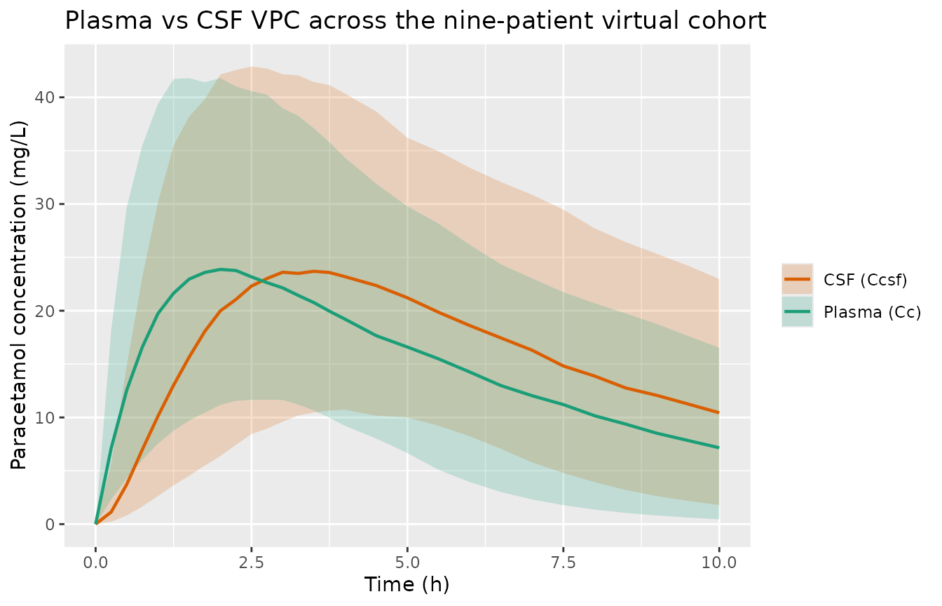
Plasma and CSF concentration-time VPCs for the nine-patient cohort (200 replicates), median and 5th-95th percentile band.
PKNCA validation
The block below runs noncompartmental analysis on the simulated
plasma and CSF profiles separately. Cmax, Tmax, AUCinf and half-life are
collected per subject and summarised across the virtual cohort. The
PKNCA formula uses output | id so per-output and
per-subject parameters are computed.
nca_plasma <- sim_typical |>
  filter(CMT == 4) |>
  transmute(id, time, conc = Cc, output = "Cc")

dose_df <- per_subject |> transmute(id, time = 0, amt = dose_mg, output = "Cc")

conc_obj <- PKNCA::PKNCAconc(nca_plasma, conc ~ time | output + id)
dose_obj <- PKNCA::PKNCAdose(dose_df,    amt  ~ time | output + id)

intervals <- data.frame(
  start = 0, end = Inf,
  cmax = TRUE, tmax = TRUE, aucinf.obs = TRUE, half.life = TRUE
)

nca_res <- PKNCA::pk.nca(PKNCA::PKNCAdata(conc_obj, dose_obj,
                                          intervals = intervals))

nca_plasma_summary <- as.data.frame(nca_res$result) |>
  filter(PPTESTCD %in% c("cmax", "tmax", "aucinf.obs", "half.life")) |>
  group_by(PPTESTCD) |>
  summarise(median = median(PPORRES, na.rm = TRUE),
            p5     = quantile(PPORRES, 0.05, na.rm = TRUE),
            p95    = quantile(PPORRES, 0.95, na.rm = TRUE),
            .groups = "drop")

knitr::kable(nca_plasma_summary,
             caption = "Plasma NCA across the virtual cohort (typical-value simulation).",
digits = 3)| PPTESTCD | median | p5 | p95 |
|---|---|---|---|
| aucinf.obs | 201.453 | 159.925 | 251.201 |
| cmax | 25.697 | 23.911 | 27.321 |
| half.life | 3.437 | 2.742 | 4.272 |
| tmax | 2.250 | 2.250 | 2.500 |
nca_csf <- sim_typical |>
  filter(CMT == 5) |>
  transmute(id, time, conc = Ccsf, output = "Ccsf")

dose_df_csf <- per_subject |> transmute(id, time = 0, amt = dose_mg, output = "Ccsf")

conc_obj_csf <- PKNCA::PKNCAconc(nca_csf, conc ~ time | output + id)
dose_obj_csf <- PKNCA::PKNCAdose(dose_df_csf, amt ~ time | output + id)

nca_res_csf <- PKNCA::pk.nca(PKNCA::PKNCAdata(conc_obj_csf, dose_obj_csf,
                                              intervals = intervals))

nca_csf_summary <- as.data.frame(nca_res_csf$result) |>
  filter(PPTESTCD %in% c("cmax", "tmax", "aucinf.obs", "half.life")) |>
  group_by(PPTESTCD) |>
  summarise(median = median(PPORRES, na.rm = TRUE),
            p5     = quantile(PPORRES, 0.05, na.rm = TRUE),
            p95    = quantile(PPORRES, 0.95, na.rm = TRUE),
            .groups = "drop")

knitr::kable(nca_csf_summary,
             caption = "CSF NCA across the virtual cohort (typical-value simulation).",
digits = 3)| PPTESTCD | median | p5 | p95 |
|---|---|---|---|
| aucinf.obs | 238.647 | 189.095 | 298.379 |
| cmax | 28.594 | 26.929 | 29.995 |
| half.life | 3.484 | 2.758 | 4.359 |
| tmax | 3.250 | 3.000 | 3.750 |
Comparison against published values
Anderson 1998 does not report Cmax, AUC, or NCA half-life tables directly; the closest published summaries are the parameter estimates themselves (Tables 2-3) and a model-predicted half-life of ln(2) * V / CL = 0.693 * 67.1 / 10.2 ~= 4.56 h for a 70 kg adult, which allometrically maps to ln(2) * (67.1 * (WT/70)^1) / (10.2 * (WT/70)^0.75) ~= 4.56 * (WT/70)^0.25 h per individual. The simulated plasma half-life above should fall within ~20 percent of that paper-implied value across the 8-50 kg cohort; large discrepancies are diagnostic of a transcription error rather than an indication to tune.
A typical-value Tmax of roughly 2-3 h on plasma and 3-4 h on CSF (one hour lagged, per equilibration teq = 0.72 h x sqrt(WT/70)^something) matches Figures 2-3 of the paper qualitatively.
Assumptions and deviations
-
Residual error is a placeholder. Anderson 1998
Methods (NONMEM paragraph) describes the residual error as “An additive
term”, while Table 3 reports
SF_C = 2.9 mmol/Lfor plasma andSF_CCSF = 2.1 mmol/Lfor CSF. The published equation 2 for the residual error (var = SF^2 * (C^PWR + V)) is the MKMODEL form and the NONMEM PWR and V terms are not reported in the paper. Taken literally as additive residual standard deviations on the paracetamol concentration scale, the reported magnitudes (2.9 and 2.1 mmol/L, equivalent to ~440 and ~320 mg/L) are 20 to 50 times larger than the observed plasma concentrations in Figures 2-3 (peak ~0.08-0.13 mmol/L, ~12-20 mg/L), which is incompatible with the additive-on-linear-scale interpretation that the Methods paragraph suggests. The most plausible reading is that “SF” in Table 3 is a software-specific scale factor (MKMODEL legacy parameterisation carried into the NONMEM column) rather than the literal additive standard deviation that nlmixr2addSdexpects. Following the precedent ofmodellib("Park_2001_ketoprofen")andmodellib("Chua_2025_mirikizumab"), this model uses a small placeholder additive residual SD on each output (addSd = addSd_Ccsf = 1.5 mg/L, ~ 10 percent of typical peak) so simulations produce plausible noise. The paper’s reported SF values are recorded in the model file’sini()comments for traceability. -
IIV is diagonal-only. Anderson 1998 Methods (NONMEM
paragraph) states that “A parameter covariance matrix was incorporated
into the structural model”, but the paper reports only the diagonal
(%CV) entries in Table 3. The full covariance matrix is not published;
the model therefore uses a diagonal-only IIV. A downstream user who
wants to layer correlations on the etas can override the omega block via
ini(...)after loading the model. -
Allometric exponents are fixed. Anderson 1998
Methods state the exponents 0.75 (CL), 1 (V) and 0.25 (teq) were
“assumed”, not estimated, so they are wrapped in
fixed()inini(). The exponent onkeq = ln(2)/teqis therefore fixed at -0.25. - ka is not allometrically scaled. The paper applies allometric scaling only to CL, V and teq; the first-order absorption rate ka is not size-dependent. The model preserves that choice.
-
Bioavailability is absorbed into apparent CL and V.
Per the paper, the symbols CL and V denote
CL / F_oralandV / F_oralfor the nasogastric route; bioavailabilityf(depot)is left at the rxode2 default of 1. -
Bannwarth and Kelley re-analyses are not extracted.
Anderson 1998 also reports two secondary fits in the same paper using
pooled summary data from the literature: an MKMODEL fit of Bannwarth et
al.’s adult propacetamol data (same structural model as Table 3, naive
pooled), and an MKMODEL PK-PD fit of Kelley et al.’s paediatric
oral-paracetamol-plus-antipyresis data (structural model extended with
an effect-compartment and sigmoid Emax). Both are naive-pooled fits with
no IIV (the reported %CVs are parameter-estimation precisions, not BSV),
so they are not packaged as separate
modellib()entries in this extraction. Their parameter values are preserved in the source paper for reproduction by future extensions. -
Reference weight is 70 kg. Anderson 1998 Methods
describes standardising all parameters to a 70 kg adult before reporting
the geometric means in Table 3, so the model’s allometric scaling uses
WT_ref = 70for every term. - No paper Cmax / AUC table. Anderson 1998 reports parameter estimates rather than NCA tables; the PKNCA section above produces simulation-based NCA values without a direct published comparator. Reviewers should sanity-check the magnitudes against Figures 2-3 of the paper rather than against a numerical table.