Ervogastat + clesacostat liver fat exposure-response (Hughes 2025)
Source:vignettes/articles/Hughes_2025_ervogastat_clesacostat.Rmd
Hughes_2025_ervogastat_clesacostat.RmdModel and source
- Citation: Hughes JH, Amin NB, Wojciechowski J, Vourvahis M. Exposure-response modeling of liver fat imaging endpoints in non-alcoholic fatty liver disease populations administered ervogastat alone and co-administered with clesacostat. CPT Pharmacometrics Syst Pharmacol. 2025;14(2):317-330.
- Article: https://doi.org/10.1002/psp4.13275 (open access, PMC11812935)
- Supplement: Data S1, which holds the PK parameter tables (Tables S3
and S4) and the three final NONMEM control streams (Code S1 ervogastat
popPK
run16, Code S2 clesacostat popPKrun100, Code S3 joint liver-fat exposure-responserun46).
Ervogastat (PF-06865571) inhibits diacylglycerol O-acyltransferase 2 and clesacostat (PF-05221304) is a liver-targeted acetyl-CoA carboxylase inhibitor; both were developed for non-alcoholic steatohepatitis (NASH). Hughes et al. built a population PK model for each drug and used the individual average steady-state concentrations from those models to drive a joint exposure-response model of two liver-fat imaging endpoints: magnetic resonance imaging proton density fat fraction (MRI-PDFF, %) and the FibroScan controlled attenuation parameter (CAP, dB/m).
The paper contributes three models, one per control stream:
# Two rxode2 warnings are expected here and are muffled by message, so any
# other warning still shows: the latent-variable random effects of the
# exposure-response model enter as `theta + s * (eta + covariates)` and are
# therefore not mu-referenced, and the typical-value solves pass several
# subjects to a model whose random effects were zeroed.
quiet_expected <- function(expr) {
  withCallingHandlers(expr, warning = function(w) {
    if (grepl("non-mu referenced|without 'omega'", conditionMessage(w))) {
      invokeRestart("muffleWarning")
    }
  })
}
models <- c(
  "Hughes_2025_ervogastat",
  "Hughes_2025_clesacostat",
  "Hughes_2025_ervogastat_clesacostat_liverfat"
)
for (m in models) {
  cat(m, ":\n  ", quiet_expected(rxode2::rxode(readModelDb(m)))$description, "\n\n", sep = "")
}
#> ℹ parameter labels from comments will be replaced by 'label()'
#> Hughes_2025_ervogastat:
#>   Two-compartment population pharmacokinetic model for oral ervogastat (PF-06865571, a diacylglycerol O-acyltransferase 2 inhibitor) in healthy participants, participants with hepatic impairment, and adults with non-alcoholic fatty liver disease (NAFLD) or presumed non-alcoholic steatohepatitis (NASH). Absorption is parallel first-order (up to a capped amount of each dose) and lagged zero-order. Apparent clearance scales allometrically with body weight and with the bioavailability-adjusted total daily dose, and is lower with hepatic impairment and in NAFLD / presumed NASH; the oral suspension raises the first-order amount cap and lowers relative bioavailability. Interindividual variability on CL/F and Vc/F; combined additive and proportional residual error with a larger proportional component in the sparsely sampled phase 2 studies. This is the ervogastat exposure model whose individual average steady-state concentrations drive the Hughes 2025 liver-fat exposure-response model (Hughes_2025_ervogastat_clesacostat_liverfat).
#> ℹ parameter labels from comments will be replaced by 'label()'
#> Hughes_2025_clesacostat:
#>   Two-compartment population pharmacokinetic model with first-order absorption for oral clesacostat (PF-05221304, a liver-targeted acetyl-CoA carboxylase inhibitor) in healthy participants, participants with hepatic impairment, and adults with non-alcoholic fatty liver disease (NAFLD) or presumed non-alcoholic steatohepatitis (NASH), alone or co-administered with ervogastat. Absorption is faster with fasting / fructose administration and with tablet formulation B; relative bioavailability is lower with fasting / fructose administration and rises stepwise at doses of 100, 200 and 240 mg. Apparent clearance scales allometrically with body weight, is higher with concomitant ervogastat, and is lower in NAFLD / presumed NASH and in SLCO1B1 intermediate or poor metabolizers. Interindividual variability on CL/F; combined additive and time-after-dose-dependent proportional residual error. This is the clesacostat exposure model whose individual average steady-state concentrations drive the Hughes 2025 liver-fat exposure-response model (Hughes_2025_ervogastat_clesacostat_liverfat).
#> ℹ parameter labels from comments will be replaced by 'label()'
#> Hughes_2025_ervogastat_clesacostat_liverfat:
#>   Joint exposure-response model for two liver-fat imaging endpoints, magnetic resonance imaging proton density fat fraction (MRI-PDFF, %) and FibroScan controlled attenuation parameter (CAP, dB/m), in adults with non-alcoholic fatty liver disease or presumed non-alcoholic steatohepatitis given ervogastat (DGAT2 inhibitor) alone or with clesacostat (ACC inhibitor). Each bounded endpoint is mapped to an unbounded scale with an Aranda-Ordaz dynamic transform-both-sides (CAP with flipped boundaries), and both transformed endpoints load on one shared latent liver-fat variable (common factor model) with an endpoint-specific baseline and scaling and an additional unique baseline random effect for CAP. The latent variable carries an exponential-onset placebo effect and a shared exponential-onset drug effect: an on/off ervogastat treatment effect that co-administered clesacostat reduces by 73.5%, plus a hyperbolic Emax effect of the individual average steady-state clesacostat concentration. Covariates: baseline ALT and age on the shared baseline, body weight on the CAP baseline, and study design and PNPLA3 genotype on the placebo effect. Observations are the transformed endpoints with additive residual error; back-transformed pdff and cap are also output.
The exposure-response model is a closed-form ($PRED)
model. Each bounded endpoint is mapped to an unbounded scale by an
Aranda-Ordaz dynamic transform-both-sides (dTBS) transformation
(Equation 1), with CAP flipped so that its dense upper boundary falls on
the flexible lower part of the transform (Equations 9 and 10). Both
transformed endpoints load on one shared latent liver-fat variable
(Equations 2-5) with endpoint-specific baselines y0k and
scalings sk:
- transformed endpoint =
y0k + sk * (latent baseline + placebo effect - drug effect), with an extra unique baseline random effect for CAP; - placebo effect =
Pmax * (1 - exp(-kpbo * t)); drug effect =(Etrt,er * on_er * (1 + Itrt,cl-er * on_cl) + Emax,cl * Cav,cl / (Cav,cl + EC50,cl)) * (1 - exp(-ktrt * t)), whereon_erandon_clare 1 when the drug is given.
The models output the transformed endpoints hpdff and
hcap (the observations, with additive residual error on the
transformed scale) and the back-transformed pdff (%) and
cap (dB/m).
Population
Table 1 of the paper summarises the three analysis populations:
| Ervogastat popPK | Clesacostat popPK | Exposure-response | |
|---|---|---|---|
| Subjects | 260 | 487 | 524 |
| Studies | 9 | 8 | 4 |
| Age, median (range), years | 49 (18-72) | 52 (19-72) | 55 (19-72) |
| Weight, median (range), kg | 91 (58.4-152) | 90 (52-170) | 93.8 (55-170) |
| Female | 27.3% | 39.6% | 50% |
| Healthy volunteers | 33.1% | 24% | - |
| Hepatic impairment (mild / moderate / severe) | 6 / 6 / 6 | 6 / 6 / 6 | - |
| NAFLD / presumed NASH | 38.8% / 21.2% | 27.1% / 45.2% | 46.6% / 53.4% |
| PNPLA3 C/C / C/G / G/G / not determined | - | - | 22.7 / 27.1 / 15.1 / 35.1% |
Studies were 11 phase 1 studies (single and multiple ascending dose,
formulation, food, hepatic impairment, Japanese participants and a
drug-drug interaction study) and three phase 2a studies; the
exposure-response analysis used the phase 1b ervogastat study in NAFLD
(NCT03513588, 2 weeks, inpatient) and the three phase 2a studies
(NCT03248882, 16 weeks; NCT03776175 and NCT04399538, 6 weeks), the phase
2a studies each starting with a 2-week placebo run-in (Table S1). The
same information is stored in each model’s population
metadata:
str(quiet_expected(rxode2::rxode(readModelDb("Hughes_2025_ervogastat_clesacostat_liverfat")))$population)
#> ℹ parameter labels from comments will be replaced by 'label()'
#> List of 14
#>  $ species       : chr "human"
#>  $ n_subjects    : int 524
#>  $ n_studies     : int 4
#>  $ n_observations: int 3100
#>  $ age_range     : chr "19-72 years"
#>  $ age_median    : chr "55 years"
#>  $ weight_range  : chr "55-170 kg"
#>  $ weight_median : chr "93.8 kg"
#>  $ sex_female_pct: num 50
#>  $ race_ethnicity: Named num [1:4] 82.8 4 10.7 2.5
#>   ..- attr(*, "names")= chr [1:4] "White" "Black" "Asian" "Other"
#>  $ disease_state : chr "Adults with NAFLD (46.6%) or presumed NASH (53.4%)"
#>  $ dose_range    : chr "Ervogastat 25-300 mg twice daily or 300 mg once daily and clesacostat 2-50 mg once daily, 2.5-15 mg twice daily"| __truncated__
#>  $ regions       : chr "United States"
#>  $ notes         : chr "Demographics from Hughes 2025 Table 1 (exposure-response column): baseline ALT median 40 IU/L (6-341), BMI medi"| __truncated__
Source trace
Every ini() value was transcribed from the final
$THETA / $OMEGA blocks of the deposited
control streams and cross-checked against the rounded values in Tables
S3, S4 and 2. Per-parameter comments in each model file give the THETA
index.
| Model | Quantity | Source |
|---|---|---|
| Ervogastat PK | Structure: 2-compartment, parallel first-order (amount-capped) and lagged zero-order absorption | Results; Supplement Equation S1; Code S1 $PK (ADVAN4, RATE = -1) |
| Ervogastat PK | ka, k0 (r1), Ak1 (amt_fo), LAG2, CL/F, Vc/F, Q/F, Vp/F | Code S1 THETA(1)-THETA(8); Table S3 |
| Ervogastat PK | Allometric exponents 0.75 and 1 (fixed), reference 70 kg | Code S1 THETA(12), THETA(13); Table S3 |
| Ervogastat PK | Effective-daily-dose power on CL/F (-0.156, reference 300 mg) | Code S1 THETA(14), EFFDOST; Table S3 |
| Ervogastat PK | Suspension effects on Ak1 (+2.34) and Frel (-0.0655) | Code S1 THETA(15), THETA(16); Table S3 |
| Ervogastat PK | Any hepatic impairment (-0.269) and NAFLD / presumed NASH (-0.185) on CL/F | Code S1 THETA(17), THETA(18); Table S3 |
| Ervogastat PK | IIV variances on CL/F (0.0953) and Vc/F (0.0997) | Code S1 $OMEGA; Table S3 (SD 0.309, 0.316) |
| Ervogastat PK | Proportional SD 0.398 (dense) / 0.711 (phase 2), additive SD 0.502 ng/mL | Code S1 THETA(9)-THETA(11); Table S3 |
| Clesacostat PK | Structure: 2-compartment, first-order absorption | Results; Code S2 $PK (ADVAN4) |
| Clesacostat PK | ka, CL/F, Vc/F, Q/F, Vp/F | Code S2 THETA(1)-THETA(5); Table S4 |
| Clesacostat PK | Allometric exponents 0.75 and 1 (fixed), reference 70 kg | Code S2 THETA(10), THETA(11); Table S4 |
| Clesacostat PK | Concomitant ervogastat on CL/F (+0.274) | Code S2 THETA(12); Table S4 |
| Clesacostat PK | Fasting / fructose on ka (+0.775) and Frel (-0.0932) | Code S2 THETA(13), THETA(14); Table S4 |
| Clesacostat PK | NAFLD / presumed NASH on CL/F (-0.293) | Code S2 THETA(15); Table S4 |
| Clesacostat PK | Dose >= 100 / 200 / 240 mg on Frel (+0.111 / +0.253 / +0.288) | Code S2 THETA(16)-THETA(18), DOSEFREL; Table S4 |
| Clesacostat PK | Tablet formulation B on ka (+1.10); SLCO1B1 IM/PM on CL/F (-0.0999) | Code S2 THETA(19), THETA(20); Table S4 |
| Clesacostat PK | IIV variance on CL/F (0.0738) | Code S2 $OMEGA; Table S4 (SD 0.269) |
| Clesacostat PK | Time-after-dose proportional SD (max 1.22, min 0.272, kRUV 0.986 1/h), additive SD 2.46 ng/mL | Code S2 THETA(6)-THETA(9); Table S4 |
| Liver fat ER | dTBS transform and back-transform; CAP flipped | Equations 1, 9, 10; Code S3 $PRED |
| Liver fat ER | Common factor structure, latent variable and scalings | Equations 2-5; Code S3 TBSLN, PMAX, EMAX |
| Liver fat ER | Baselines -1.16 / 5.05 and alpha 4.92 / 32.1 (fixed) | Code S3 THETA(1), THETA(2), THETA(10), THETA(11); Table 2 |
| Liver fat ER | Placebo and drug onset half-lives 49.1 and 18.8 days | Code S3 THETA(3), THETA(4); Table 2 |
| Liver fat ER | Pmax 0.393, Etrt,er 1.27, Emax,cl 2.32, EC50,cl 389 ng/mL, Itrt,cl-er -0.735 | Code S3 THETA(5)-THETA(9); Table 2 |
| Liver fat ER | Residual SDs 0.205 (MRI-PDFF) and 5.35 (CAP) on the transformed scales | Code S3 THETA(12), THETA(13); Table 2 |
| Liver fat ER | Scalings s_MRI 0.698 and -s_CAP 2.77 | Code S3 THETA(14), THETA(15); Table 2 |
| Liver fat ER | ALT (0.575, ref 40 IU/L) and age (-0.564, ref 51 y) on the shared baseline; weight (3.80, ref 92 kg) on the CAP baseline | Code S3 THETA(16), THETA(22), THETA(17); Equation 12; Table 2 |
| Liver fat ER | Inpatient study (-2.74) and PNPLA3 C/C, C/G, G/G (-1.00, -0.694, -0.0835) on Pmax | Code S3 THETA(18)-THETA(21); Table 2 |
| Liver fat ER | IIV variances 1 (fixed), 1.78, 0.919 (shared baseline, unique CAP baseline, Pmax) | Code S3 $OMEGA; Table 2 (SD 1.00, 1.33, 0.959) |
| Liver fat ER | Placebo clock from baseline observation in phase 2a studies, from first dose otherwise; drug clock from first dose | Code S3 PTIME, DTIME |
Ervogastat and clesacostat pharmacokinetics
Virtual cohorts
Two ervogastat cohorts reproduce the phase 1b study in adults with NAFLD (NCT03513588: 50 or 300 mg twice daily, immediate-release tablet, 14 days) and two clesacostat cohorts reproduce the phase 2a co-administration studies (NCT04399538: 10 mg twice daily, tablet B, presumed NASH; NCT03776175: 15 mg twice daily, tablet A, NAFLD), each with 100 participants. Body weight is drawn from a normal distribution matching Table 1 (mean 92.5 kg, SD 18.2 kg, truncated to the observed range).
Each ervogastat administration is two dose records with the same
amount: one into depot (first-order part) and one into
central with rate = -1, so the zero-order rate
is the modelled r1 and the split between the two parts
comes from f(depot) and f(central). This
reproduces the NONMEM data layout of Code S1.
set.seed(2025)
rxode2::rxSetSeed(2025)
n_pk <- 100
tau <- 12
n_dose <- 28
dose_times <- seq(0, by = tau, length.out = n_dose)
obs_times <- sort(unique(c(seq(0, 300, by = 12), seq(312, 324, by = 0.25))))

draw_wt <- function(n) pmin(pmax(rnorm(n, 92.5, 18.2), 52), 170)

ervo_events <- function(dose, id0) {
  ids <- id0 + seq_len(n_pk)
  cov <- data.frame(
    id = ids, WT = draw_wt(n_pk),
    DOSE_ERVOGASTAT_MG = dose, DOSE_ERVOGASTAT_MGD = 2 * dose,
    FORM_ERVOGASTAT_SUSP = 0, HEPIMP = 0, DIS_NAFLD = 1, STUDY_PHASE2 = 0,
    treatment = paste0("Ervogastat ", dose, " mg BID")
  )
  dep <- tidyr::crossing(cov, time = dose_times) |>
    mutate(amt = dose, evid = 1, cmt = "depot", rate = 0)
  cen <- tidyr::crossing(cov, time = dose_times) |>
    mutate(amt = dose, evid = 1, cmt = "central", rate = -1)
  obs <- tidyr::crossing(cov, time = obs_times) |>
    mutate(amt = 0, evid = 0, cmt = "central", rate = 0)
  bind_rows(dep, cen, obs) |> arrange(id, time, desc(evid))
}

cles_events <- function(dose, form_b, id0, label) {
  ids <- id0 + seq_len(n_pk)
  cov <- data.frame(
    id = ids, WT = draw_wt(n_pk),
    DOSE_CLESACOSTAT_MG = dose, CONMED_ERVOGASTAT = 1, FED = 1,
    FORM_CLESACOSTAT_TABLETB = form_b, DIS_NAFLD = 1,
    SLCO1B1_PM_IM = rbinom(n_pk, 1, 0.214),
    treatment = label
  )
  dos <- tidyr::crossing(cov, time = dose_times) |>
    mutate(amt = dose, evid = 1, cmt = "depot")
  obs <- tidyr::crossing(cov, time = obs_times) |>
    mutate(amt = 0, evid = 0, cmt = "central")
  bind_rows(dos, obs) |> arrange(id, time, desc(evid))
}

ev_ervo <- bind_rows(ervo_events(50, 0), ervo_events(300, 1000))
ev_cles <- bind_rows(
  cles_events(10, 1, 2000, "Clesacostat 10 mg BID (tablet B)"),
  cles_events(15, 0, 3000, "Clesacostat 15 mg BID (tablet A)")
)
Simulation
mod_ervo <- readModelDb("Hughes_2025_ervogastat")
mod_cles <- readModelDb("Hughes_2025_clesacostat")

sim_ervo <- rxode2::rxSolve(mod_ervo, ev_ervo, keep = "treatment", returnType = "data.frame")
#> ℹ parameter labels from comments will be replaced by 'label()'
sim_cles <- rxode2::rxSolve(mod_cles, ev_cles, keep = "treatment", returnType = "data.frame")
#> ℹ parameter labels from comments will be replaced by 'label()'

pk_all <- bind_rows(
  sim_ervo |> select(id, time, Cc, treatment, cl, f = frel),
  sim_cles |> select(id, time, Cc, treatment, cl, f = fdepot)
)
pk_all |>
  filter(time >= 312) |>
  mutate(tad = time - 312) |>
  group_by(treatment, tad) |>
  summarise(
    med = median(Cc), lo = quantile(Cc, 0.05), hi = quantile(Cc, 0.95),
    .groups = "drop"
  ) |>
  ggplot(aes(tad, med)) +
  geom_ribbon(aes(ymin = lo, ymax = hi), alpha = 0.25) +
  geom_line() +
  facet_wrap(~treatment, scales = "free_y") +
  labs(
    x = "Time after the day-14 morning dose (h)", y = "Plasma concentration (ng/mL)",
    caption = "Median and 90% interval of 100 simulated participants per regimen (individual predictions)."
  )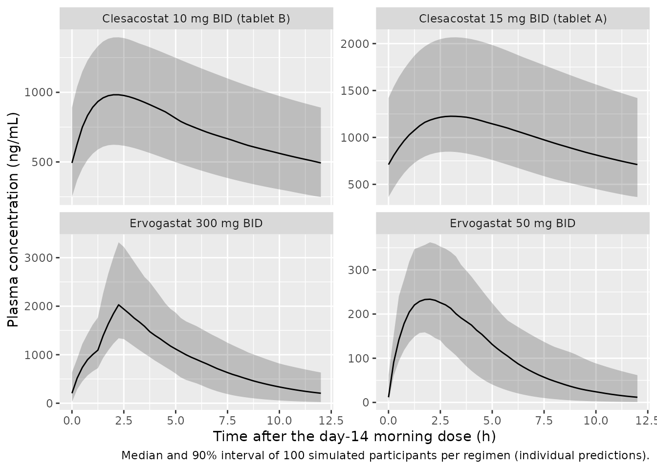
The ervogastat profile shows the two absorption phases: a fast first-order input of up to 197 mg of each dose and, after a 1.24 h lag, a zero-order input of the remainder at 101 mg/h. At 50 mg the cap exceeds the dose, so almost the entire dose is absorbed first-order.
NCA (PKNCA)
The steady-state dosing interval after the day-14 morning dose
(312-324 h) is analysed with PKNCA. The paper reports no NCA, so the
check is internal: at steady state AUCtau must equal
F * dose / (CL/F) for each participant, which tests the
dose split between the two ervogastat absorption pathways, the
rate-defined zero-order input, the bioavailability terms and the
mg-to-ng/mL scaling.
conc <- pk_all |>
  filter(time >= 312, !is.na(Cc)) |>
  select(id, time, Cc, treatment)
dose_df <- bind_rows(
  ev_ervo |> filter(evid == 1, cmt == "depot"),
  ev_cles |> filter(evid == 1)
) |>
  select(id, time, amt, treatment)

conc_obj <- PKNCA::PKNCAconc(conc, Cc ~ time | treatment + id)
dose_obj <- PKNCA::PKNCAdose(dose_df, amt ~ time | treatment + id)
intervals <- data.frame(start = 312, end = 324, auclast = TRUE, cmax = TRUE, tmax = TRUE, cmin = TRUE)
nca <- PKNCA::pk.nca(PKNCA::PKNCAdata(conc_obj, dose_obj, intervals = intervals))
nca_res <- as.data.frame(nca$result)

nca_res |>
  filter(PPTESTCD %in% c("auclast", "cmax", "tmax", "cmin")) |>
  group_by(treatment, PPTESTCD) |>
  summarise(median = signif(median(PPORRES), 3), .groups = "drop") |>
  tidyr::pivot_wider(names_from = PPTESTCD, values_from = median) |>
  dplyr::rename(
    Regimen = treatment, "AUCtau (ng*h/mL)" = auclast, "Cmax (ng/mL)" = cmax,
    "Tmax (h)" = tmax, "Cmin (ng/mL)" = cmin
  ) |>
knitr::kable(caption = "Median steady-state NCA over the day-14 morning dosing interval.")| Regimen | AUCtau (ng*h/mL) | Cmax (ng/mL) | Cmin (ng/mL) | Tmax (h) |
|---|---|---|---|---|
| Clesacostat 10 mg BID (tablet B) | 8670 | 983 | 493.0 | 2.25 |
| Clesacostat 15 mg BID (tablet A) | 12000 | 1230 | 711.0 | 3.25 |
| Ervogastat 300 mg BID | 10500 | 2030 | 206.0 | 2.25 |
| Ervogastat 50 mg BID | 1340 | 237 | 11.7 | 1.75 |
indiv <- pk_all |>
  filter(time == 312) |>
  distinct(id, treatment, cl, f)
dose_amt <- dose_df |> distinct(id, amt)
auc_chk <- nca_res |>
  filter(PPTESTCD == "auclast") |>
  inner_join(indiv, by = c("id", "treatment")) |>
  inner_join(dose_amt, by = "id") |>
  mutate(
    auc_expected = 1000 * f * amt / cl,
    ratio = PPORRES / auc_expected
  )
auc_chk |>
  group_by(treatment) |>
  summarise(
    "median AUCtau / (F x dose / CL)" = round(median(ratio), 4),
    "10th-90th percentile" = paste(round(quantile(ratio, c(0.1, 0.9)), 4), collapse = " - "),
    .groups = "drop"
  ) |>
knitr::kable()| treatment | median AUCtau / (F x dose / CL) | 10th-90th percentile |
|---|---|---|
| Clesacostat 10 mg BID (tablet B) | 0.9996 | 0.9994 - 0.9996 |
| Clesacostat 15 mg BID (tablet A) | 0.9998 | 0.9997 - 0.9998 |
| Ervogastat 300 mg BID | 0.9992 | 0.9985 - 0.9995 |
| Ervogastat 50 mg BID | 0.9983 | 0.9972 - 0.9991 |
Liver fat exposure-response
mod_er <- quiet_expected(rxode2::rxode(readModelDb("Hughes_2025_ervogastat_clesacostat_liverfat")))
#> ℹ parameter labels from comments will be replaced by 'label()'
mod_er_typ <- quiet_expected(rxode2::zeroRe(mod_er))
Replicating Figure 4 (typical-value covariate effects)
Figure 4 shows the population-typical MRI-PDFF and CAP over 6 weeks of ervogastat / clesacostat 300/10 mg twice daily for a reference participant and for the 5th and 95th percentiles (or each category) of each covariate. The reference values printed in the figure legends are age 55 years, ALT 54 IU/L and body weight 93 kg. The reference PNPLA3 genotype is not stated; the C/C curve of the PNPLA3 panel coincides with the reference curves of the other panels, so C/C is used. The clesacostat average concentration is the typical value for a 93 kg participant with presumed NASH given 10 mg twice daily with food and with ervogastat, from the clesacostat model.
cav_typ <- function(dose_mg, n_per_day, wt, slco = 0) {
  ev <- data.frame(
    id = 1, time = c(0, 1), evid = c(1, 0), amt = c(dose_mg, 0), cmt = c("depot", "central"),
    WT = wt, DOSE_CLESACOSTAT_MG = dose_mg, CONMED_ERVOGASTAT = 1, FED = 1,
    FORM_CLESACOSTAT_TABLETB = 1, DIS_NAFLD = 1, SLCO1B1_PM_IM = slco
  )
  s <- rxode2::rxSolve(rxode2::zeroRe(mod_cles), ev, returnType = "data.frame")
  1000 * s$fdepot[1] * dose_mg * n_per_day / (24 * s$cl[1])
}
cav_ref <- cav_typ(10, 2, 93)
#> ℹ parameter labels from comments will be replaced by 'label()'
#> ℹ omega/sigma items treated as zero: 'etalcl'
cav_ref
#> [1] 676.7092
weeks <- seq(0, 6, by = 0.25)
ref <- data.frame(
  ALT = 54, AGE = 55, WT = 93, PNPLA3_CC = 1, PNPLA3_CG = 0, PNPLA3_GG = 0,
  STUDY_PHASE2 = 1, STUDY_NCT03513588 = 0, T_SCAN_TO_DOSE = 0,
  CAV_ERVOGASTAT = 1, CAV_CLESACOSTAT = cav_ref
)
scen <- list(
  list(panel = "Age (years)", level = "29", AGE = 29),
  list(panel = "Age (years)", level = "55"),
  list(panel = "Age (years)", level = "68", AGE = 68),
  list(panel = "ALT (IU/L)", level = "25", ALT = 25),
  list(panel = "ALT (IU/L)", level = "54"),
  list(panel = "ALT (IU/L)", level = "135", ALT = 135),
  list(panel = "Body weight (kg)", level = "67", WT = 67),
  list(panel = "Body weight (kg)", level = "93"),
  list(panel = "Body weight (kg)", level = "127", WT = 127),
  list(panel = "PNPLA3", level = "C/C"),
  list(panel = "PNPLA3", level = "C/G", PNPLA3_CC = 0, PNPLA3_CG = 1),
  list(panel = "PNPLA3", level = "G/G", PNPLA3_CC = 0, PNPLA3_GG = 1)
)
fig4_ev <- bind_rows(lapply(seq_along(scen), function(i) {
  s <- scen[[i]]
  d <- ref
  for (nm in setdiff(names(s), c("panel", "level"))) d[[nm]] <- s[[nm]]
  data.frame(id = i, time = weeks * 168, d, panel = s$panel, level = s$level)
}))
fig4 <- quiet_expected(rxode2::rxSolve(mod_er_typ, fig4_ev, keep = c("panel", "level"), returnType = "data.frame"))
#> ℹ omega/sigma items treated as zero: 'etabsl', 'etabsl_hcap', 'etapmax'

fig4 |>
  select(panel, level, time, "MRI-PDFF (%)" = pdff, "CAP (dB/m)" = cap) |>
  pivot_longer(c("MRI-PDFF (%)", "CAP (dB/m)"), names_to = "endpoint") |>
  mutate(
    endpoint = factor(endpoint, c("MRI-PDFF (%)", "CAP (dB/m)")),
    level = factor(level, unique(fig4$level))
  ) |>
  ggplot(aes(time / 168, value, colour = level)) +
  geom_line() +
  facet_wrap(panel ~ endpoint, scales = "free_y", ncol = 2) +
  labs(
    x = "Time after first dose (weeks)", y = "Predicted liver fat", colour = NULL,
    caption = "Replicates Figure 4 of Hughes 2025 (typical values, 300/10 mg BID)."
  )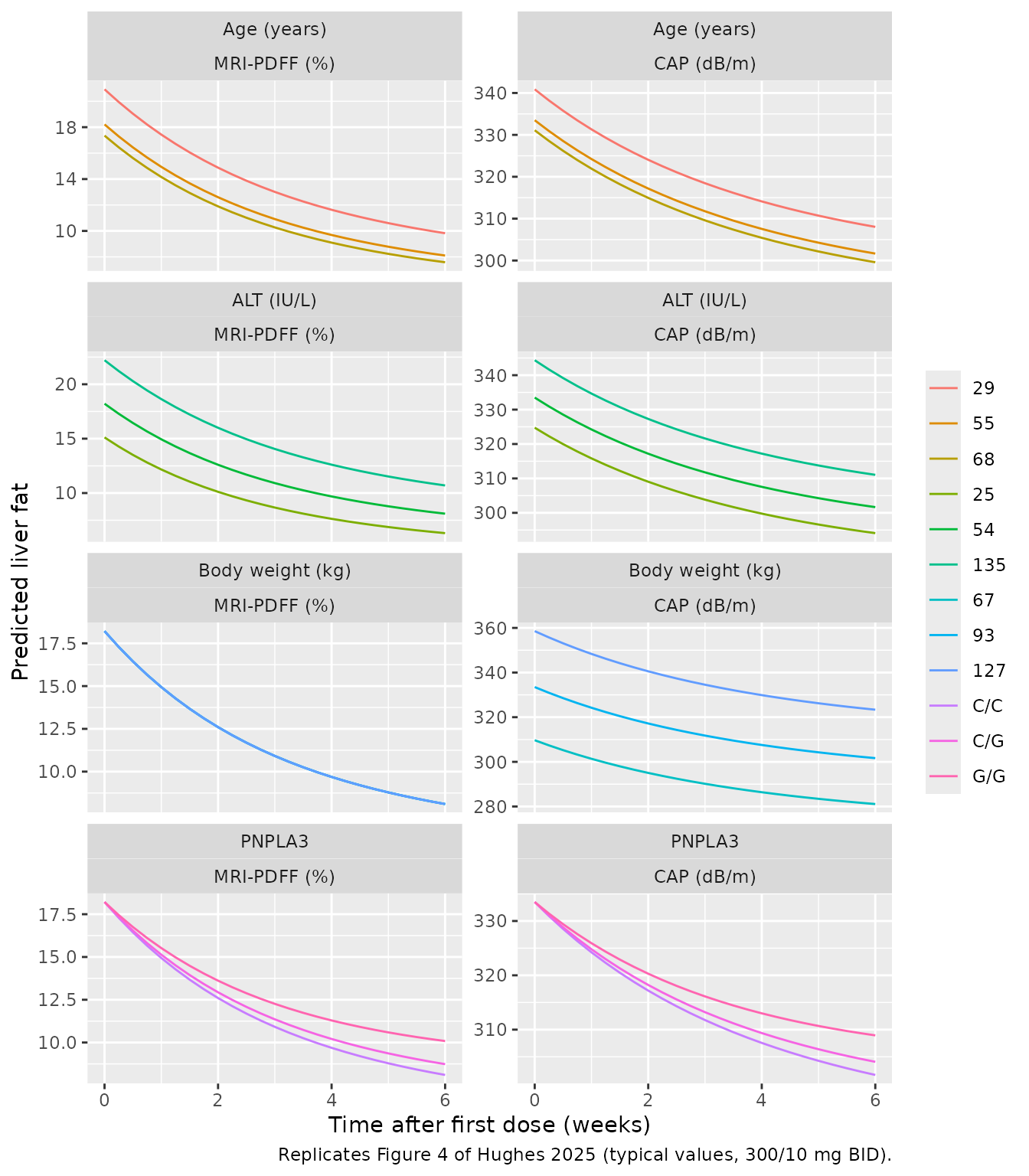
The maintainers read the start and end of selected curves off Figure 4 (to about the line width, so roughly +/- 0.3 % PDFF and +/- 2 dB/m):
fig4_pub <- tibble::tribble(
  ~curve, ~endpoint, ~week, ~published,
  "Reference", "pdff", 0, 18.2,
  "Reference", "pdff", 6, 8.0,
  "Reference", "cap", 0, 333,
  "Reference", "cap", 6, 301,
  "Age 29", "pdff", 0, 21.0,
  "Age 29", "pdff", 6, 9.8,
  "ALT 25", "pdff", 0, 15.0,
  "ALT 25", "pdff", 6, 6.4,
  "ALT 135", "pdff", 0, 22.3,
  "ALT 135", "pdff", 6, 10.7,
  "Weight 67", "cap", 0, 309,
  "Weight 67", "cap", 6, 280,
  "Weight 127", "cap", 0, 358,
  "Weight 127", "cap", 6, 325,
  "PNPLA3 G/G", "pdff", 6, 9.9
)
key <- c(
  "Reference" = "Age (years)|55", "Age 29" = "Age (years)|29", "ALT 25" = "ALT (IU/L)|25",
  "ALT 135" = "ALT (IU/L)|135", "Weight 67" = "Body weight (kg)|67",
  "Weight 127" = "Body weight (kg)|127", "PNPLA3 G/G" = "PNPLA3|G/G"
)
sim_pts <- fig4 |>
  mutate(key = paste(panel, level, sep = "|"), week = time / 168) |>
  filter(week %in% c(0, 6)) |>
  select(key, week, pdff, cap) |>
  pivot_longer(c(pdff, cap), names_to = "endpoint", values_to = "simulated")
fig4_cmp <- fig4_pub |>
  mutate(key = key[curve]) |>
  inner_join(sim_pts, by = c("key", "endpoint", "week")) |>
  mutate(simulated = round(simulated, 1), pct_diff = round(100 * (simulated - published) / published, 1))
fig4_cmp |>
  select(Curve = curve, Endpoint = endpoint, Week = week, Published = published, Simulated = simulated, "% difference" = pct_diff) |>
knitr::kable()| Curve | Endpoint | Week | Published | Simulated | % difference |
|---|---|---|---|---|---|
| Reference | pdff | 0 | 18.2 | 18.2 | 0.0 |
| Reference | pdff | 6 | 8.0 | 8.1 | 1.2 |
| Reference | cap | 0 | 333.0 | 333.5 | 0.2 |
| Reference | cap | 6 | 301.0 | 301.7 | 0.2 |
| Age 29 | pdff | 0 | 21.0 | 20.9 | -0.5 |
| Age 29 | pdff | 6 | 9.8 | 9.8 | 0.0 |
| ALT 25 | pdff | 0 | 15.0 | 15.1 | 0.7 |
| ALT 25 | pdff | 6 | 6.4 | 6.3 | -1.6 |
| ALT 135 | pdff | 0 | 22.3 | 22.2 | -0.4 |
| ALT 135 | pdff | 6 | 10.7 | 10.7 | 0.0 |
| Weight 67 | cap | 0 | 309.0 | 309.7 | 0.2 |
| Weight 67 | cap | 6 | 280.0 | 281.1 | 0.4 |
| Weight 127 | cap | 0 | 358.0 | 358.6 | 0.2 |
| Weight 127 | cap | 6 | 325.0 | 323.4 | -0.5 |
| PNPLA3 G/G | pdff | 6 | 9.9 | 10.1 | 2.0 |
stopifnot(
  # Baselines test the transforms, scalings and covariate terms exactly.
  all(abs(fig4_cmp$pct_diff[fig4_cmp$week == 0]) < 3),
  # Week-6 values add the placebo and drug terms and the onset half-lives.
  abs(median(fig4_cmp$pct_diff[fig4_cmp$week == 6])) < 5
)
All baselines agree to within the reading precision of the figure, confirming the Aranda-Ordaz back-transformation (including the flipped CAP boundaries), the endpoint scalings and the ALT, age and weight terms. The week-6 values agree to within a few percent; with C/G as the reference genotype instead, the reference week-6 MRI-PDFF would be about 8.7%, above the published curve.
Replicating Table 3 (clinical trial simulation of NCT04399538)
Table 3 gives the placebo-corrected percent change from baseline at
week 6 for the NCT04399538 design: presumed NASH, a 2-week placebo
run-in starting at the baseline imaging visit (Day -14), then 6 weeks of
ervogastat / clesacostat with clesacostat tablet B taken with food. The
paper sampled covariates from the observed NCT04399538 participants,
which are not published; here 200 virtual participants draw ALT, age and
weight from distributions matching the exposure-response column of Table
1, PNPLA3 genotype from its Table 1 frequencies, and SLCO1B1
intermediate-or-poor function with the Table 1 frequency (19.1%). The
same 200 participants, with the same random effects, appear in every
arm, so the placebo correction is a paired comparison. Each
participant’s clesacostat average steady-state concentration comes from
the clesacostat model with interindividual variability
(Cav = 1000 * F * daily dose / (24 * CL/F)); the ervogastat
effect only needs the ervogastat concentration to be positive.
set.seed(4399538)
rxode2::rxSetSeed(4399538)
n_er <- 200
arms <- tibble::tribble(
  ~arm, ~ervo, ~cles_dose, ~per_day,
  "Placebo", 0, 0, 0,
  "25/10 mg BID", 25, 10, 2,
  "100/10 mg BID", 100, 10, 2,
  "300/20 mg QD", 300, 20, 1,
  "300/10 mg BID", 300, 10, 2,
  "300/5 mg BID", 300, 5, 2,
  "300/2.5 mg BID", 300, 2.5, 2
)
draw_er <- function(n) {
  g <- sample(c("CC", "CG", "GG", "ND"), n, replace = TRUE, prob = c(22.7, 27.1, 15.1, 35.1))
  data.frame(
    ALT = pmin(pmax(rlnorm(n, log(40), 0.62), 6), 341),
    AGE = pmin(pmax(rnorm(n, 53, 11.4), 19), 72),
    WT = pmin(pmax(rnorm(n, 96.5, 19), 55), 170),
    SLCO1B1_PM_IM = rbinom(n, 1, 0.191),
    PNPLA3_CC = as.integer(g == "CC"), PNPLA3_CG = as.integer(g == "CG"),
    PNPLA3_GG = as.integer(g == "GG")
  )
}

# One cohort shared by every arm, so that the placebo correction compares the
# same participants. The exposure-response random effects are drawn here from
# the model's omega and passed as data columns to the zero-random-effect model.
om <- mod_er$omega
pop <- data.frame(subj = seq_len(n_er), draw_er(n_er))
pop$etabsl <- rnorm(n_er, 0, sqrt(om["etabsl", "etabsl"]))
pop$etabsl_hcap <- rnorm(n_er, 0, sqrt(om["etabsl_hcap", "etabsl_hcap"]))
pop$etapmax <- rnorm(n_er, 0, sqrt(om["etapmax", "etapmax"]))

# Individual clesacostat CL/F and F from the clesacostat model, with its own
# interindividual variability (one 10 mg dose and one observation per
# participant; every simulated dose is below the 100 mg Frel step).
pk_ev <- pop |>
  transmute(
    id = subj, WT, SLCO1B1_PM_IM,
    DOSE_CLESACOSTAT_MG = 10, CONMED_ERVOGASTAT = 1, FED = 1, FORM_CLESACOSTAT_TABLETB = 1, DIS_NAFLD = 1
  )
pk_ev <- bind_rows(
  pk_ev |> mutate(time = 0, evid = 1, amt = 10, cmt = "depot"),
  pk_ev |> mutate(time = 1, evid = 0, amt = 0, cmt = "central")
) |>
  arrange(id, time)
cles_ind <- rxode2::rxSolve(mod_cles, pk_ev, returnType = "data.frame") |>
  group_by(id) |>
  slice(1) |>
  ungroup() |>
  select(subj = id, cl, fdepot)

er_cohort <- tidyr::crossing(pop, arms) |>
  left_join(cles_ind, by = "subj") |>
  mutate(
    id = match(arm, arms$arm) * 1000 + subj,
    CAV_CLESACOSTAT = ifelse(cles_dose > 0, 1000 * fdepot * cles_dose * per_day / (24 * cl), 0),
    CAV_ERVOGASTAT = as.numeric(ervo > 0),
    STUDY_PHASE2 = 1, STUDY_NCT03513588 = 0, T_SCAN_TO_DOSE = 14 * 24
  )
er_cohort |>
  filter(CAV_CLESACOSTAT > 0) |>
  group_by(arm) |>
  summarise("median clesacostat Cav (ng/mL)" = signif(median(CAV_CLESACOSTAT), 3)) |>
knitr::kable()| arm | median clesacostat Cav (ng/mL) |
|---|---|
| 100/10 mg BID | 688 |
| 25/10 mg BID | 688 |
| 300/10 mg BID | 688 |
| 300/2.5 mg BID | 172 |
| 300/20 mg QD | 688 |
| 300/5 mg BID | 344 |
t_week6 <- (14 + 42) * 24
er_ev <- bind_rows(
  er_cohort |> mutate(time = 0),
  er_cohort |> mutate(time = t_week6)
) |>
  arrange(id, time) |>
  select(id, time, arm, ALT, AGE, WT, starts_with("PNPLA3"), starts_with("eta"), CAV_ERVOGASTAT, CAV_CLESACOSTAT, STUDY_PHASE2, STUDY_NCT03513588, T_SCAN_TO_DOSE)
er_sim <- quiet_expected(rxode2::rxSolve(mod_er_typ, er_ev, keep = "arm", returnType = "data.frame"))
#> ℹ omega/sigma items treated as zero: 'etabsl', 'etabsl_hcap', 'etapmax'

chg <- er_sim |>
  group_by(id, arm) |>
  summarise(
    pdff = 100 * (last(pdff) - first(pdff)) / first(pdff),
    cap = 100 * (last(cap) - first(cap)) / first(cap),
    .groups = "drop"
  ) |>
  group_by(arm) |>
  summarise(pdff = mean(pdff), cap = mean(cap), .groups = "drop")
pbo <- chg |> filter(arm == "Placebo")
tab3_sim <- chg |>
  filter(arm != "Placebo") |>
  mutate(pdff = pdff - pbo$pdff, cap = cap - pbo$cap)

tab3_pub <- tibble::tribble(
  ~arm, ~pdff_obs, ~pdff_pub, ~cap_obs, ~cap_pub,
  "25/10 mg BID", -52.4, -45.7, -6.45, -7.35,
  "100/10 mg BID", -56.6, -45.4, -1.69, -7.24,
  "300/20 mg QD", -58.8, -45.9, -5.60, -7.40,
  "300/10 mg BID", -45.8, -45.6, -3.57, -7.48,
  "300/5 mg BID", NA, -37.4, NA, -5.57,
  "300/2.5 mg BID", NA, -28.9, NA, -4.29
)
tab3 <- tab3_pub |>
  inner_join(tab3_sim, by = "arm") |>
  mutate(
    pdff = round(pdff, 1), cap = round(cap, 2),
    pdff_diff = round(100 * (pdff - pdff_pub) / abs(pdff_pub), 1),
    cap_diff = round(100 * (cap - cap_pub) / abs(cap_pub), 1)
  )
tab3 |>
  select(
    Regimen = arm, "MRI-PDFF observed" = pdff_obs, "MRI-PDFF published prediction" = pdff_pub,
    "MRI-PDFF simulated" = pdff, "MRI-PDFF % diff" = pdff_diff,
    "CAP observed" = cap_obs, "CAP published prediction" = cap_pub,
    "CAP simulated" = cap, "CAP % diff" = cap_diff
  ) |>
knitr::kable(caption = "Placebo-corrected percent change from baseline at week 6 (replicates Table 3 of Hughes 2025; observed values are adjusted geometric least-squares means).")| Regimen | MRI-PDFF observed | MRI-PDFF published prediction | MRI-PDFF simulated | MRI-PDFF % diff | CAP observed | CAP published prediction | CAP simulated | CAP % diff |
|---|---|---|---|---|---|---|---|---|
| 25/10 mg BID | -52.4 | -45.7 | -47.3 | -3.5 | -6.45 | -7.35 | -7.61 | -3.5 |
| 100/10 mg BID | -56.6 | -45.4 | -47.3 | -4.2 | -1.69 | -7.24 | -7.61 | -5.1 |
| 300/20 mg QD | -58.8 | -45.9 | -47.3 | -3.1 | -5.60 | -7.40 | -7.61 | -2.8 |
| 300/10 mg BID | -45.8 | -45.6 | -47.3 | -3.7 | -3.57 | -7.48 | -7.61 | -1.7 |
| 300/5 mg BID | NA | -37.4 | -38.8 | -3.7 | NA | -5.57 | -6.02 | -8.1 |
| 300/2.5 mg BID | NA | -28.9 | -29.9 | -3.5 | NA | -4.29 | -4.47 | -4.2 |
stopifnot(
  # A transcription error in Emax, EC50, the interaction or a scaling moves
  # every arm by tens of percent.
  abs(median(c(tab3$pdff_diff, tab3$cap_diff))) < 10,
  quantile(abs(c(tab3$pdff_diff, tab3$cap_diff)), 0.9) < 20
)
The simulated placebo-corrected changes match the published model predictions closely, including the loss of efficacy as the clesacostat dose falls from 10 to 2.5 mg twice daily. Like the published predictions, they cannot distinguish the ervogastat doses: the ervogastat effect is an on/off treatment effect because its EC50 was not identifiable.
Assumptions and deviations
-
Ervogastat dose records. Each administration needs
two dose records with the same amount (one into
depot, one intocentralwithrate = -1), and the covariateDOSE_ERVOGASTAT_MGmust equal that amount; Code S1 builds the data the same way. Code S1 caps the first-order fraction at 0.999 when the amount cap exceeds the dose (Supplement Equation S1 prints 1); the model follows the control stream. - Hepatic impairment classification. The ervogastat model pools mild, moderate and severe hepatic impairment into one effect; the paper does not name the grading system.
-
NAFLD indicator.
DIS_NAFLD = 1for NAFLD and for presumed NASH, which the models pool into one effect. Confirmed NASH (Code S1 / S2 category 6) is not in the data and is not part of the effect. -
Food in the clesacostat model.
FED = 1is the reference (standard meal, high-fat meal, or dosing without regard to food); fasting and fructose administration are bothFED = 0. -
SLCO1B1 and PNPLA3 references. For clesacostat,
SLCO1B1 ‘not determined’ is pooled with extensive function (Code S2). In
the exposure-response model the PNPLA3 reference is the participants
without a genotype, so C/C carries its own indicator
(
PNPLA3_CC). -
Exposure-response time axis. Model time is time
after the baseline imaging visit.
T_SCAN_TO_DOSEis the time from that visit to the first dose (336 h for a Day -14 baseline). The placebo clock runs from the baseline visit in the three phase 2a studies (STUDY_PHASE2 = 1) and from the first dose otherwise; the drug clock always runs from the first dose. - Boundary observations. The estimation used a censored likelihood for CAP values at the 400 dB/m boundary and adjusted boundary values by 0.5 dB/m; that is part of fitting, not simulation, and is not encoded. The three CAP values at 100 dB/m were excluded as outliers before the final fit.
- Table 3 cohort. The paper sampled covariates from the observed NCT04399538 participants and included parameter uncertainty and residual error over 1000 simulated trials of 15 participants per arm. Here the covariates come from Table 1 distributions, there is no parameter uncertainty, and the percent changes use individual predictions without residual error, so only the central values are compared.
- Figure 4 reference genotype. The reference PNPLA3 genotype of Figure 4 is not stated; C/C reproduces the reference curves.