Polymyxin B in ECMO (Xu 2024)
Source:vignettes/articles/Xu_2024_polymyxinB.Rmd
Xu_2024_polymyxinB.RmdModel and source
mod_meta <- nlmixr2est::nlmixr(readModelDb("Xu_2024_polymyxinB"))$meta
#> ℹ parameter labels from comments will be replaced by 'label()'- Citation: Xu M, Chen N, Yu YW, Pan XY, Li T. Pharmacokinetic Changes and Influencing Factors of Polymyxin B in Different ECMO Modes. Infect Drug Resist. 2024;17:5815-5825. doi:10.2147/IDR.S486169
- Description: Two-compartment IV infusion population PK model for polymyxin B (summed PMB1 + PMB2) in 11 critically ill adults on venoarterial or venovenous ECMO with carbapenem-resistant Gram-negative infections (Xu 2024). Clearance is 3.75 L/h at an ECMO blood flow of 3.48 L/min and falls linearly by 32.1% per L/min of additional flow, CL = 3.75 * (1 - 0.321 * (Q_ECMO - 3.48)). The central volume is 20.41 L in a patient receiving CRRT and 52.5% smaller (9.69 L) without CRRT. Peripheral volume 9.86 L and intercompartmental clearance 3.82 L/h carry no covariates. Exponential IIV on CL (omega^2 = 0.038) and on the central volume (omega^2 = 0.062); additive residual error 0.361 mg/L.
- Article (DOI): https://doi.org/10.2147/IDR.S486169
This vignette validates the packaged Xu_2024_polymyxinB
model, a two-compartment population PK model for polymyxin B (PMB1 +
PMB2 summed) developed in Phoenix NLME from 132 steady-state plasma
samples in 11 critically ill adults supported by venoarterial (8) or
venovenous (3) extracorporeal membrane oxygenation (ECMO). Two
covariates were retained: the ECMO blood flow rate, which enters
clearance as a linear centred term, and continuous renal replacement
therapy (CRRT), which enters the central volume.
mod <- readModelDb("Xu_2024_polymyxinB")
mod
#> function() {
#>   description <- "Two-compartment IV infusion population PK model for polymyxin B (summed PMB1 + PMB2) in 11 critically ill adults on venoarterial or venovenous ECMO with carbapenem-resistant Gram-negative infections (Xu 2024). Clearance is 3.75 L/h at an ECMO blood flow of 3.48 L/min and falls linearly by 32.1% per L/min of additional flow, CL = 3.75 * (1 - 0.321 * (Q_ECMO - 3.48)). The central volume is 20.41 L in a patient receiving CRRT and 52.5% smaller (9.69 L) without CRRT. Peripheral volume 9.86 L and intercompartmental clearance 3.82 L/h carry no covariates. Exponential IIV on CL (omega^2 = 0.038) and on the central volume (omega^2 = 0.062); additive residual error 0.361 mg/L."
#>   reference <- "Xu M, Chen N, Yu YW, Pan XY, Li T. Pharmacokinetic Changes and Influencing Factors of Polymyxin B in Different ECMO Modes. Infect Drug Resist. 2024;17:5815-5825. doi:10.2147/IDR.S486169"
#>   vignette <- "Xu_2024_polymyxinB"
#>   units <- list(time = "h", dosing = "mg", concentration = "mg/L")
#>
#>   # Total polymyxin B (PMB1 + PMB2 summed) in plasma by LC-MS/MS (Xu 2024
#>   # Drug Assay section); the peripheral compartment is the model's tissue
#>   # distribution space.
#>   compartmentData <- list(
#>     central = list(analyte = "polymyxinB", units = "mg", specimen = "plasma", verified = TRUE),
#>     peripheral1 = list(analyte = "polymyxinB", units = "mg", specimen = "tissue", verified = TRUE)
#>   )
#>
#>   covariateData <- list(
#>     Q_ECMO = list(
#>       description = "ECMO circuit blood flow rate",
#>       units = "L/min",
#>       type = "continuous",
#>       reference_category = NULL,
#>       notes = "Source covariate 'speadECMO' in the final-model CL equation, defined in the Table 2 footnote as 'spead of ECMO (L/min)'; the L/min unit identifies it as the delivered blood flow rather than the pump speed (Table 1 reports pump speed separately in RPM, median 3500). Table 1 median (IQR) 3.60 (3.00, 3.65) L/min. Enters CL as the linear centred form 1 + dCLdspeedECMO * (Q_ECMO - 3.48), with 3.48 L/min the centring value printed in the equation (not the Table 1 median of 3.60). Treated as a per-subject value at the steady-state sampling occasion; the paper does not describe flow as time-varying. Because the effect is linear with a negative slope (-0.321 per L/min), predicted CL reaches zero at Q_ECMO = 3.48 + 1/0.321 = 6.60 L/min; do not extrapolate far outside the observed 3.0-3.65 L/min interquartile range.",
#>       source_name = "speadECMO"
#>     ),
#>     RRT_CRRT_STATUS = list(
#>       description = "Subject-level binary indicator for continuous renal replacement therapy during the PK sampling period",
#>       units = "(binary)",
#>       type = "binary",
#>       reference_category = 0,
#>       notes = "Source covariate CRRT. Table 1: 8/11 (72.73%) received CRRT, all of it continuous venovenous haemodialysis (CVVHD; Ultraflux AV1000S) for anuria, connected in the ECMO circuit (outflow at the post-oxygenator, inflow at the pre-oxygenator line). The paper estimates the effect in the Phoenix 'dVdCRRT0' parameterization, V = tvV * (1 + dVdCRRT0 * (if no CRRT)), so the typical central volume of 20.41 L is the CRRT value and the -0.525 coefficient applies to patients WITHOUT CRRT. Encoded here as (1 + e_nocrrt_vc * (1 - RRT_CRRT_STATUS)). Direction: CRRT is associated with a larger central volume, as the Discussion states ('patients receiving CRRT-ECMO had significantly increased the central compartment').",
#>       source_name = "CRRT"
#>     )
#>   )
#>
#>   covariatesDataExcluded <- list(
#>     AGE = list(
#>       description = "Subject age",
#>       units = "years",
#>       type = "continuous",
#>       notes = "The Results text says 'CRRT and age were identified as the covariates for V', and the Table 2 abbreviation list defines 'dVdage, fixed parameter coefficient of age (year) to V', but neither the printed final-model V equation nor the Table 2 parameter rows contain an age term or estimate. The printed equation is taken as the final model, so age is not carried. Table 1 median (IQR) 56 (48, 64) years; the Results prose gives 60 (53.50-62.50)."
#>     )
#>   )
#>
#>   population <- list(
#>     species = "human",
#>     n_subjects = 11L,
#>     n_studies = 1L,
#>     age_range = "Adults (>= 18 years); Table 1 median (IQR) 56 (48, 64) years (the Results prose reports 60, 53.50-62.50)",
#>     weight_range = "Median (IQR) 60 (57.05, 66.00) kg; BSA 1.69 (1.68, 1.79) m^2 (Table 1)",
#>     sex_female_pct = 27.27,
#>     race_ethnicity = "Not reported (single-centre Chinese ICU cohort)",
#>     disease_state = "Heart or respiratory failure requiring ECMO (8 VA-ECMO, 3 VV-ECMO; SOFA >= 2) with infection by carbapenem-resistant A. baumannii (7), K. pneumoniae (6) or P. aeruginosa (3), polymyxin B MIC 0.5 mg/L. Pneumonia 9/11, bloodstream infection 4/11. Median APACHE II 14, SOFA 10. ECMO duration median 16.18 days.",
#>     dose_range = "Loading dose 200-300 mg on day 1, then 100-150 mg (2.5-3 mg/kg/day) at the treating physician's discretion, each dose in 50 mL saline as a 1-h infusion. Sampling at steady state (after more than four doses) at 1, 1.5, 2, 4, 8 and 12 h after the start of infusion, pre- and post-oxygenator.",
#>     regions = "China (First Affiliated Hospital of Zhejiang University School of Medicine; single centre)",
#>     renal_function = "8/11 on CVVHD for anuria. Table 1 CrCL median (IQR) 79.70 (33.33, 94.89) mL/min; serum creatinine 137.27 (71.00, 184.50), labelled mg/dL but clearly umol/L.",
#>     ecmo = "Rotaflow centrifugal pump with polymethylpentene oxygenator (MAQUET), PVC tubing, 600 mL saline prime. Pump speed median 3500 (3000, 3770) RPM; blood flow 3.60 (3.00, 3.65) L/min.",
#>     notes = "Prospective study, January-December 2021. 132 plasma samples (66 pre- and 66 post-oxygenator; no significant difference between sites, Figure 1). Estimation: Phoenix NLME 8.1, FOCE; pcVPC with 1000 replicates and 1000-sample bootstrap."
#>   )
#>
#>   ini({
#>     # Structural parameters: Xu 2024 Table 2, 'Final Model Estimate, Mean'
#>     # column. The reference patient receives CRRT and has an ECMO blood flow
#>     # of 3.48 L/min (final-model CL and V equations).
#>     lcl <- log(3.75); label("Clearance at Q_ECMO = 3.48 L/min (L/h)") # Table 2: tvCL = 3.75 L/h (CV 6.98%; bootstrap median 3.74, 95% CI 1.59-4.34)
#>     lvc <- log(20.41); label("Central volume of distribution with CRRT (L)") # Table 2: tvV = 20.41 L (CV 17.1%; bootstrap median 20.47, 95% CI 12.82-27.89)
#>     lvp <- log(9.86); label("Peripheral volume of distribution (L)") # Table 2: tvVp = 9.86 L (CV 53.4%; bootstrap median 10.34, 95% CI 4.06-24.34)
#>     lq <- log(3.82); label("Intercompartmental clearance (L/h)") # Table 2: tvQ = 3.82 L/h (CV 42.1%; bootstrap median 4.19, 95% CI 1.83-10.49)
#>
#>     # Covariate effects (final-model equations printed in the Results)
#>     e_q_ecmo_cl <- -0.321; label("Fractional change in CL per L/min of ECMO blood flow above 3.48 L/min (1/(L/min))") # Table 2: dCLdspeedECMO = -0.321 (bootstrap median -0.315, 95% CI -0.710 to 0.00120); CL equation: tvCL * (1 + (speadECMO - 3.48 L/min) * dCLdspeadECMO)
#>     e_nocrrt_vc <- -0.525; label("Fractional change in central volume without CRRT (unitless)") # Table 2: dVdCRRT0 = -0.525 (bootstrap median -0.553, 95% CI -0.769 to -0.207); V equation: tvV * (1 + dVdCRRTO * (if no CRRT))
#>
#>     # Between-subject variability: Table 2 rows 'omega2 V' and 'omega2 CL',
#>     # footnoted as variances; exponential IIV per Methods. No covariance
#>     # term is reported.
#>     etalcl ~ 0.038 # Table 2: omega2 CL = 0.038 (bootstrap median 0.049)
#>     etalvc ~ 0.062 # Table 2: omega2 V = 0.062 (bootstrap median 0.058)
#>
#>     # Residual variability: Table 2 'stdev0' = 0.361. The Results select 'the
#>     # two-compartment model with an additive option', and the Figure 3 pcVPC
#>     # lower prediction band dips below zero, consistent with an additive
#>     # (not proportional) error in mg/L.
#>     addSd <- 0.361; label("Additive residual error (mg/L)") # Table 2: stdev0 = 0.361 (CV 12.0%; bootstrap median 0.351, 95% CI 0.256-0.447)
#>   })
#>   model({
#>     # Individual parameters (Xu 2024 final-model equations)
#>     cl <- exp(lcl + etalcl) * (1 + e_q_ecmo_cl * (Q_ECMO - 3.48))
#>     vc <- exp(lvc + etalvc) * (1 + e_nocrrt_vc * (1 - RRT_CRRT_STATUS))
#>     vp <- exp(lvp)
#>     q <- exp(lq)
#>
#>     kel <- cl / vc
#>     k12 <- q / vc
#>     k21 <- q / vp
#>
#>     # Two-compartment disposition; polymyxin B given as a 1-h IV infusion
#>     # into the central compartment. Dose in mg and volume in L give mg/L.
#>     d/dt(central) <- -kel * central - k12 * central + k21 * peripheral1
#>     d/dt(peripheral1) <- k12 * central - k21 * peripheral1
#>
#>     Cc <- central / vc
#>     Cc ~ add(addSd)
#>   })
#> }
#> <environment: 0x55564a1df4a0>
Population
tibble::tribble(
  ~Characteristic,             ~Value,
  "Subjects",                  "11 (132 plasma samples, pre- and post-oxygenator)",
  "Sex",                       "8 male (72.73%), 3 female (27.27%)",
  "Age (years)",               "56 (48, 64)",
  "Weight (kg)",               "60 (57.05, 66.00)",
  "BSA (m^2)",                 "1.69 (1.68, 1.79)",
  "CrCL (mL/min)",             "79.70 (33.33, 94.89)",
  "Albumin (g/L)",             "34.00 (30.55, 36.20)",
  "CRRT",                      "8 (72.73%), all CVVHD",
  "ECMO mode (VA / VV)",       "8 / 3",
  "ECMO pump speed (RPM)",     "3500 (3000, 3770)",
  "ECMO blood flow (L/min)",   "3.60 (3.00, 3.65)",
  "ECMO duration (days)",      "16.18 (8.50, 23.00)",
  "APACHE II / SOFA",          "14 (9.50, 18.00) / 10 (4.00, 11.50)"
) |>
knitr::kable(caption = "Xu 2024 Table 1; continuous values are median (IQR).")| Characteristic | Value |
|---|---|
| Subjects | 11 (132 plasma samples, pre- and post-oxygenator) |
| Sex | 8 male (72.73%), 3 female (27.27%) |
| Age (years) | 56 (48, 64) |
| Weight (kg) | 60 (57.05, 66.00) |
| BSA (m^2) | 1.69 (1.68, 1.79) |
| CrCL (mL/min) | 79.70 (33.33, 94.89) |
| Albumin (g/L) | 34.00 (30.55, 36.20) |
| CRRT | 8 (72.73%), all CVVHD |
| ECMO mode (VA / VV) | 8 / 3 |
| ECMO pump speed (RPM) | 3500 (3000, 3770) |
| ECMO blood flow (L/min) | 3.60 (3.00, 3.65) |
| ECMO duration (days) | 16.18 (8.50, 23.00) |
| APACHE II / SOFA | 14 (9.50, 18.00) / 10 (4.00, 11.50) |
All patients had carbapenem-resistant A. baumannii, K. pneumoniae or P. aeruginosa infection (polymyxin B MIC 0.5 mg/L). They received a 200-300 mg loading dose on day 1, then 100-150 mg (2.5-3 mg/kg/day), each dose as a 1-hour infusion. Samples were drawn at steady state (after more than four doses) at 1, 1.5, 2, 4, 8 and 12 h after the start of an infusion. Pre- and post-oxygenator concentrations did not differ (Figure 1), so the two sampling sites are pooled in the model.
Source trace
tibble::tribble(
  ~Quantity,                    ~`Model file`,     ~Value,          ~`Source location`,
  "Clearance (Q_ECMO 3.48)",    "lcl",             "3.75 L/h",      "Table 2 tvCL; CL equation",
  "Central volume (CRRT)",      "lvc",             "20.41 L",       "Table 2 tvV; V equation",
  "Peripheral volume",          "lvp",             "9.86 L",        "Table 2 tvVp",
  "Intercompartmental CL",      "lq",              "3.82 L/h",      "Table 2 tvQ",
  "ECMO flow slope on CL",      "e_q_ecmo_cl",     "-0.321 per L/min", "Table 2 dCLdspeedECMO; CL equation",
  "No-CRRT effect on V",        "e_nocrrt_vc",     "-0.525",        "Table 2 dVdCRRT0; V equation",
  "IIV on CL (variance)",       "etalcl",          "0.038",         "Table 2 omega2 CL",
  "IIV on V (variance)",        "etalvc",          "0.062",         "Table 2 omega2 V",
  "Additive residual SD",       "addSd",           "0.361 mg/L",    "Table 2 stdev0; Results 'additive option'",
  "Structural model",           "d/dt(central), d/dt(peripheral1)", "2-cmt", "Results, OFV 109.9 vs 126.6 for 1-cmt",
  "Flow centring value",        "3.48",            "3.48 L/min",    "CL equation",
  "Infusion duration",          "dur = 1",         "1 h",           "Methods, Drug Regimens"
) |>
knitr::kable(caption = "Source trace for every ini() value and structural choice.")| Quantity | Model file | Value | Source location |
|---|---|---|---|
| Clearance (Q_ECMO 3.48) | lcl | 3.75 L/h | Table 2 tvCL; CL equation |
| Central volume (CRRT) | lvc | 20.41 L | Table 2 tvV; V equation |
| Peripheral volume | lvp | 9.86 L | Table 2 tvVp |
| Intercompartmental CL | lq | 3.82 L/h | Table 2 tvQ |
| ECMO flow slope on CL | e_q_ecmo_cl | -0.321 per L/min | Table 2 dCLdspeedECMO; CL equation |
| No-CRRT effect on V | e_nocrrt_vc | -0.525 | Table 2 dVdCRRT0; V equation |
| IIV on CL (variance) | etalcl | 0.038 | Table 2 omega2 CL |
| IIV on V (variance) | etalvc | 0.062 | Table 2 omega2 V |
| Additive residual SD | addSd | 0.361 mg/L | Table 2 stdev0; Results ‘additive option’ |
| Structural model | d/dt(central), d/dt(peripheral1) | 2-cmt | Results, OFV 109.9 vs 126.6 for 1-cmt |
| Flow centring value | 3.48 | 3.48 L/min | CL equation |
| Infusion duration | dur = 1 | 1 h | Methods, Drug Regimens |
The final-model equations printed in the Results are
CL = tvCL x (1 + (speadECMO - 3.48 L/min) x dCLdspeadECMO) x exp(nCL)
V  = tvV  x (1 + dVdCRRTO x (if no CRRT)) x exp(nV)
In this Phoenix parameterization the typical central volume of 20.41 L belongs to a patient on CRRT and the -0.525 coefficient applies to patients without CRRT, so CRRT is associated with a larger central volume, as the Discussion states.
Typical parameter values by covariate
typ <- tidyr::expand_grid(
  RRT_CRRT_STATUS = c(1, 0),
  Q_ECMO = c(3.0, 3.48, 3.6, 4.0, 5.0)
) |>
  mutate(
    `CL (L/h)` = 3.75 * (1 - 0.321 * (Q_ECMO - 3.48)),
    `V (L)` = 20.41 * (1 - 0.525 * (1 - RRT_CRRT_STATUS)),
    CRRT = ifelse(RRT_CRRT_STATUS == 1, "CRRT", "no CRRT")
  )
typ |>
  select(CRRT, `ECMO flow (L/min)` = Q_ECMO, `CL (L/h)`, `V (L)`) |>
knitr::kable(digits = 2, caption = "Typical CL and central volume across the covariate range.")| CRRT | ECMO flow (L/min) | CL (L/h) | V (L) |
|---|---|---|---|
| CRRT | 3.00 | 4.33 | 20.41 |
| CRRT | 3.48 | 3.75 | 20.41 |
| CRRT | 3.60 | 3.61 | 20.41 |
| CRRT | 4.00 | 3.12 | 20.41 |
| CRRT | 5.00 | 1.92 | 20.41 |
| no CRRT | 3.00 | 4.33 | 9.69 |
| no CRRT | 3.48 | 3.75 | 9.69 |
| no CRRT | 3.60 | 3.61 | 9.69 |
| no CRRT | 4.00 | 3.12 | 9.69 |
| no CRRT | 5.00 | 1.92 | 9.69 |
The packaged model must reproduce these closed-form typical values
exactly. zeroRe() removes the random effects, so the
comparison is pure arithmetic.
mod_typ <- zeroRe(mod)
#> ℹ parameter labels from comments will be replaced by 'label()'
typ_ev <- typ |>
  mutate(id = row_number(), time = 0, amt = 0, evid = 0, cmt = "central") |>
  select(id, time, amt, evid, cmt, Q_ECMO, RRT_CRRT_STATUS)
typ_sim <- rxSolve(mod_typ, typ_ev, returnType = "data.frame", addDosing = FALSE)
#> ℹ omega/sigma items treated as zero: 'etalcl', 'etalvc'
#> Warning: multi-subject simulation without without 'omega'
stopifnot(
  max(abs(typ_sim$cl - typ$`CL (L/h)`)) < 1e-8,
  max(abs(typ_sim$vc - typ$`V (L)`)) < 1e-8
)
flow_grid <- tibble(Q_ECMO = seq(2.5, 5, by = 0.05)) |>
  mutate(cl = 3.75 * (1 - 0.321 * (Q_ECMO - 3.48)))
ggplot(flow_grid, aes(Q_ECMO, cl)) +
  annotate("rect", xmin = 3.0, xmax = 3.65, ymin = -Inf, ymax = Inf, alpha = 0.15) +
  geom_line() +
  geom_point(data = tibble(Q_ECMO = 3.48, cl = 3.75), colour = "red") +
  labs(x = "ECMO blood flow (L/min)", y = "Typical CL (L/h)")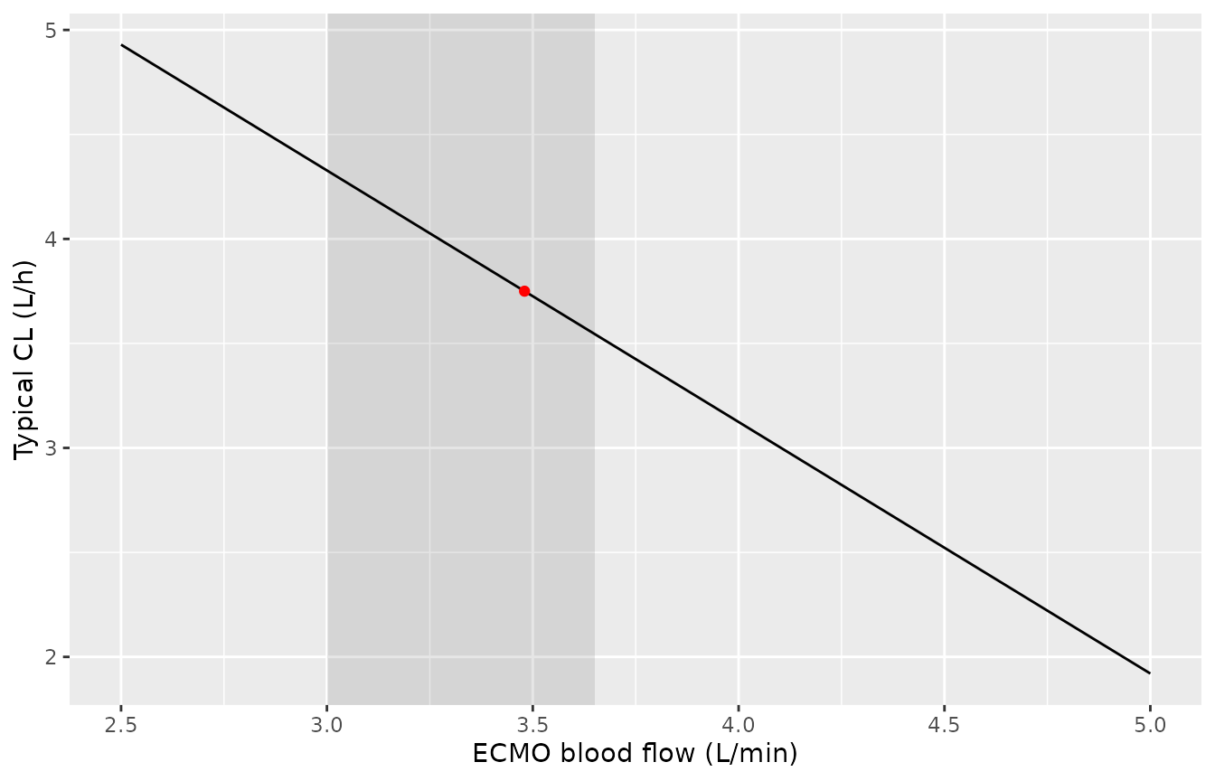
Typical clearance against ECMO blood flow (Xu 2024 CL equation). The shaded band is the Table 1 interquartile range of flow (3.00-3.65 L/min).
Virtual cohort
Covariates are drawn to resemble Table 1: CRRT with probability 8/11, and ECMO blood flow from a normal distribution with mean 3.4 L/min and SD 0.45 L/min truncated to 2.5-4.5 L/min (Table 1 reports only the median and IQR). Two maintenance regimens bracket the reported dosing: 50 mg and 75 mg every 12 h (100 and 150 mg/day), each preceded by a 200 mg loading dose and given as 1-h infusions. Ten maintenance doses bring every subject to steady state, and the final interval is sampled densely.
set.seed(20241227)
rxSetSeed(20241227)
n_per_arm <- 200L
tau <- 12
n_maint <- 10L
arms <- tibble(treatment = c("50 mg q12h", "75 mg q12h"), maint = c(50, 75))

cov_df <- tidyr::expand_grid(arm_i = seq_len(nrow(arms)), j = seq_len(n_per_arm)) |>
  mutate(
    id = row_number(),
    treatment = arms$treatment[arm_i],
    maint = arms$maint[arm_i],
    RRT_CRRT_STATUS = rbinom(n(), 1, 8 / 11),
    Q_ECMO = pmin(pmax(rnorm(n(), 3.4, 0.45), 2.5), 4.5)
  )

dose_times <- c(0, tau * seq_len(n_maint))
t_last <- max(dose_times)
obs_times <- t_last + c(0, seq(0.25, tau, by = 0.25))

dose_rows <- cov_df |>
  tidyr::expand_grid(time = dose_times) |>
  mutate(
    amt = ifelse(time == 0, 200, maint),
    evid = 1L,
    dur = 1
  )
obs_rows <- cov_df |>
  tidyr::expand_grid(time = obs_times) |>
  mutate(amt = 0, evid = 0L, dur = 0)
events <- bind_rows(dose_rows, obs_rows) |>
  mutate(cmt = "central") |>
  arrange(id, time, desc(evid)) |>
  select(id, time, amt, evid, dur, cmt, treatment, Q_ECMO, RRT_CRRT_STATUS)

sim <- rxSolve(mod, events, returnType = "data.frame", addDosing = FALSE,
               keep = c("treatment")) |>
  mutate(tad = time - t_last)
#> ℹ parameter labels from comments will be replaced by 'label()'
Replicate Figure 3 (prediction-corrected VPC)
Figure 3 of Xu 2024 is a prediction-corrected VPC of the steady-state interval. The points below are the observed median of that figure, digitised by the maintainers at the paper’s sampling times; they are approximate and are shown for orientation only. The paper does not report the individual maintenance doses, so both simulated regimens are drawn.
fig3_obs <- tibble(
  tad = c(1.25, 2, 4, 7),
  Cc = c(3.1, 2.3, 1.75, 1.0)
)
vpc <- sim |>
  group_by(treatment, tad) |>
  summarise(
    p05 = quantile(Cc, 0.05),
    p50 = median(Cc),
    p95 = quantile(Cc, 0.95),
    .groups = "drop"
  )
ggplot(vpc, aes(tad, p50, colour = treatment, fill = treatment)) +
  geom_ribbon(aes(ymin = p05, ymax = p95), alpha = 0.15, colour = NA) +
  geom_line() +
  geom_point(data = fig3_obs, aes(tad, Cc), inherit.aes = FALSE) +
  labs(x = "Time after dose (h)", y = "Polymyxin B concentration (mg/L)",
       colour = NULL, fill = NULL)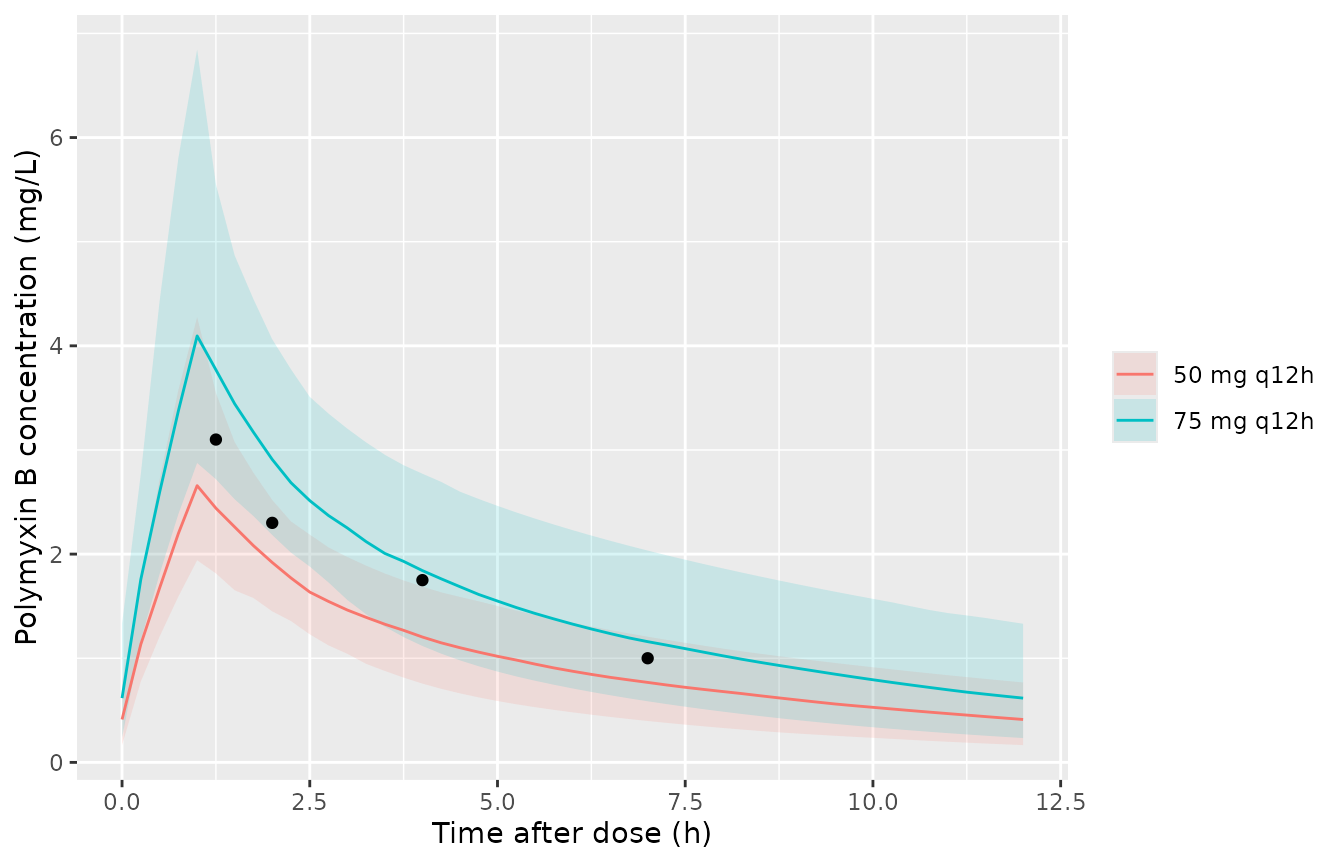
Simulated steady-state concentrations (median and 5th-95th percentile band) for the two maintenance regimens. Black points: observed median read from Xu 2024 Figure 3. Replicates Figure 3 of Xu 2024.
The digitised observed median falls between the two simulated regimens, which is consistent with the 100-150 mg/day dosing the Methods describe.
PKNCA validation
Steady-state NCA over the final 12-h interval, by regimen.
sim_nca <- sim |>
  filter(!is.na(Cc)) |>
  mutate(time = tad) |>
  select(id, time, Cc, treatment)
dose_nca <- events |>
  filter(evid == 1, time == t_last) |>
  mutate(time = 0) |>
  select(id, time, amt, treatment)

conc_obj <- PKNCA::PKNCAconc(sim_nca, Cc ~ time | treatment + id,
                             concu = "mg/L", timeu = "h")
dose_obj <- PKNCA::PKNCAdose(dose_nca, amt ~ time | treatment + id,
                             doseu = "mg")
intervals <- data.frame(
  start = 0, end = tau,
  cmax = TRUE, tmax = TRUE, cmin = TRUE, auclast = TRUE, cav = TRUE
)
nca_res <- PKNCA::pk.nca(PKNCA::PKNCAdata(conc_obj, dose_obj, intervals = intervals))
summary(nca_res)
#>  Interval Start Interval End  treatment   N AUClast (h*mg/L) Cmax (mg/L)
#>               0           12 50 mg q12h 200      12.7 [24.0] 2.78 [26.4]
#>               0           12 75 mg q12h 200      19.6 [25.6] 4.23 [27.0]
#>   Cmin (mg/L)          Tmax (h)  Cav (mg/L)
#>  0.388 [56.7] 1.00 [1.00, 1.00] 1.06 [24.0]
#>  0.615 [59.9] 1.00 [1.00, 1.00] 1.63 [25.6]
#>
#> Caption: AUClast, Cmax, Cmin, Cav: geometric mean and geometric coefficient of variation; Tmax: median and range; N: number of subjects
Mass balance at steady state
At steady state the AUC over one interval equals dose / CL for every subject. Both sides use the same drawn parameters, so the difference is only the trapezoidal error of the 0.25-h grid.
cl_by_id <- sim |> distinct(id, cl)
auc_chk <- as.data.frame(nca_res) |>
  filter(PPTESTCD == "auclast") |>
  select(id, treatment, auclast = PPORRES) |>
  left_join(cl_by_id, by = "id") |>
  left_join(dose_nca |> select(id, amt), by = "id") |>
  mutate(pct_diff = 100 * (auclast - amt / cl) / (amt / cl))
summary(auc_chk$pct_diff)
#>     Min.  1st Qu.   Median     Mean  3rd Qu.     Max.
#> -0.22316 -0.04201 -0.02004 -0.03162 -0.01085  0.36296
stopifnot(max(abs(auc_chk$pct_diff)) < 1)
Comparison with the published Css,avg
Xu 2024 reports Css,avg (AUC0-tau / tau from WinNonlin) only by microbiological outcome: 2.26 +/- 0.72 mg/L in the clearance group and 1.25 +/- 0.24 mg/L in the uncleared group (Results and Figure 4). Because those groups are defined by outcome rather than by regimen, the side-by-side table below is context rather than a like-for-like NCA comparison.
cav_sim <- as.data.frame(nca_res) |>
  filter(PPTESTCD == "cav") |>
  group_by(treatment) |>
  summarise(
    median = median(PPORRES),
    p05 = quantile(PPORRES, 0.05),
    p95 = quantile(PPORRES, 0.95),
    .groups = "drop"
  )
bind_rows(
  cav_sim |>
    transmute(Source = paste("Simulated,", treatment),
              Value = sprintf("%.2f (%.2f-%.2f)", median, p05, p95)),
  tibble(Source = c("Xu 2024, clearance group", "Xu 2024, uncleared group"),
         Value = c("2.26 +/- 0.72", "1.25 +/- 0.24"))
) |>
  rename(`Css,avg (mg/L)` = Value) |>
knitr::kable(caption = "Simulated median (5th-95th percentile) Css,avg against the published outcome-group mean +/- SD.")| Source | Css,avg (mg/L) |
|---|---|
| Simulated, 50 mg q12h | 1.07 (0.74-1.47) |
| Simulated, 75 mg q12h | 1.63 (1.13-2.44) |
| Xu 2024, clearance group | 2.26 +/- 0.72 |
| Xu 2024, uncleared group | 1.25 +/- 0.24 |
cav75 <- cav_sim$median[cav_sim$treatment == "75 mg q12h"]
stopifnot(cav75 > 1.25, cav75 < 2.26)
The 150 mg/day regimen gives a median Css,avg between the two published group means, as expected for a cohort dosed at 100-150 mg/day whose individual exposures span both groups.
Assumptions and deviations
-
Age is not carried. The Results text says “CRRT and
age were identified as the covariates for V”, and the Table 2
abbreviations define a
dVdagecoefficient, but neither the printed V equation nor the Table 2 parameter rows contain an age term or estimate. The printed final-model equation is implemented; age is recorded incovariatesDataExcluded. -
ECMO flow, not pump speed. The CL covariate is
printed as
speadECMOwith units of L/min, which identifies it as the delivered blood flow (Table 1 reports pump speed separately in RPM). It is mapped toQ_ECMO. The centring value 3.48 L/min is the one in the printed equation, not the Table 1 median of 3.60 L/min. The Discussion at one point links ECMO flow to the volume of distribution; the equation and Table 2 put the effect on CL, which is what is implemented. - Linear flow effect. With a slope of -0.321 per L/min the typical CL reaches zero at 6.60 L/min. The observed flows were 3.0-3.65 L/min (IQR); do not extrapolate far outside that range.
-
Residual error is additive. Table 2 reports a
single
stdev0of 0.361. The Results select “the two-compartment model with an additive option”, and the lower prediction band of the Figure 3 VPC falls below zero, which only an additive error produces. It is encoded as an additive SD in mg/L. - IIV. Table 2 reports variances of 0.062 (V) and 0.038 (CL) for an exponential model; no covariance is reported. No IIV is reported on Vp or Q.
- Dosing in the simulations. The Methods give “100-150 mg (2.5-3 mg/kg/day)” without stating the interval; the 12-h sampling schedule and the Figure 3 concentrations agree with 50-75 mg every 12 h, which is what is simulated. The loading dose is taken as 200 mg.
- Covariate distribution. Table 1 gives only the median and IQR of ECMO flow; the truncated normal used for the virtual cohort is a maintainers’ choice.
- Table 1 inconsistencies. Serum creatinine is labelled mg/dL but the values (median 137.27) are umol/L; the Results prose gives CrCL the same numbers as serum creatinine and an age median of 60 (53.50-62.50) against Table 1’s 56 (48, 64). The number of patients with bacterial clearance is 7 in the Results and 6 in Table 1. None of these enters the model.
-
Convention-check note.
checkModelConventions()warns thate_q_ecmo_cl“looks like a reversed-order covariate effect” because its first tokenqis also a PK parameter name. The covariate isQ_ECMO, so the name is in the canonicale_<cov>_<param>order, matchinge_q_ecmo_cl_1ohminKim_2026_midazolam_ecmo.