hUGT1A1-modRNA for Crigler-Najjar syndrome type 1 (Apgar 2018)
Source:vignettes/articles/Apgar_2018_ALXN1540.Rmd
Apgar_2018_ALXN1540.RmdModel and source
Apgar and colleagues built a quantitative systems pharmacology (QSP) model of ALXN1540, a modified messenger RNA encoding human UGT1A1 delivered as a lipid nanoparticle (LNP), as a treatment for Crigler-Najjar syndrome type 1 (CN1). The model was calibrated to Gunn rats, the UGT1A1-deficient animal model of CN1, and then translated to CN1 patients to support first-in-human dose selection.
The paper presents two KroneckerBio model files, and this package therefore ships two model objects:
rat <- rxode2::rxode(readModelDb("Apgar_2018_ALXN1540_rat_qsp"))
human <- rxode2::rxode(readModelDb("Apgar_2018_ALXN1540_human_qsp"))- Citation: Apgar JF, Tang JP, Singh P, Balasubramanian N, Burke JM, Hodges MR, Lasaro MA, Lin L, Millard BL, Moore K, Jun LS, Sobolov S, Wilkins AK, Gao X. Quantitative Systems Pharmacology Model of hUGT1A1-modRNA Encoding for the UGT1A1 Enzyme to Treat Crigler-Najjar Syndrome Type 1. CPT Pharmacometrics Syst Pharmacol. 2018;7(6):404-412. doi:10.1002/psp4.12301. Author names as corrected by the Corrigendum, CPT Pharmacometrics Syst Pharmacol. 2020;9:185, doi:10.1002/psp4.12484 (author-name corrections only; no parameter, equation or unit is revised). Rate constants and plasma volume from Table 1 (Gunn rat column); reaction network from Supplementary Model S1 (Gunn Rat KroneckerBio Model File).
- Article: https://doi.org/10.1002/psp4.12301
- Supplementary material (reaction networks, Table S1): https://europepmc.org/article/PMC/PMC6391595
The two files are not a base/final pair: they differ in structure as well as in parameter values, so each is extracted as published (see Structural differences below).
Gunn rat model. QSP (preclinical, Gunn rat). Mechanistic model of ALXN1540 (hUGT1A1-modRNA in a lipid nanoparticle) for Crigler-Najjar syndrome type 1. Eleven states chain lipid-nanoparticle plasma disposition and hepatocyte attachment, endocytosis and endosomal escape, to cytoplasmic mRNA, UGT1A1 protein translation and turnover, and enzymatic glucuronidation of bilirubin to mono- and diglucuronide with their faster elimination. Amounts in nmol; second-order terms use amount/plasma-volume concentrations in nM.
CN1 human model. QSP. Humanized (Crigler-Najjar syndrome type 1) translation of the ALXN1540 (hUGT1A1-modRNA lipid nanoparticle) mechanistic model used for first-in-human dose projection. Twelve states chain lipid-nanoparticle plasma disposition and hepatocyte attachment, endocytosis and endosomal escape, to cytoplasmic mRNA, UGT1A1 protein translation and turnover, and two-step enzymatic glucuronidation of bilirubin via explicit enzyme-substrate complexes. Biophysical and cellular rate constants are carried over from the Gunn rat fit; bilirubin production and clearance are human CN1 values. Amounts in nmol; second-order terms use amount/plasma-volume concentrations in nM.
Population
The Gunn rat model was calibrated against three studies in Gunn-UGT1a1j/BluHsdRrrc rats: a single-dose 0.3 mg/kg i.v. PK/PD study in adult (N = 4-5) and juvenile (N = 5) animals; a repeat-dose PD study in adult animals at 0.1, 0.2 and 0.5 mg/kg Q2W and 0.5 mg/kg Q4W for five doses, with a 0.5 mg/kg Q2W luciferase-mRNA vehicle control (N = 4-5 per time point); and an escalating single-dose PD study at 0.1, 0.2 and 0.5 mg/kg used as a naive prediction check (N = 4-6 per time point). Male and female, adolescent and adult animals were enrolled; because “no clear gender or age differences were noted in the PK data”, all groups were pooled for calibration. Body weights recorded in the deposited single-dose dataset span 155-262 g (adults) and 70-116 g (juveniles).
The human model is a forward projection, not a fit – no CN1 patients were dosed. Biophysical and cellular parameters are carried over from the rat estimates, and only bilirubin production and clearance are humanized.
str(rat$population, give.attr = FALSE)
#> List of 7
#>  $ species      : chr "rat (Gunn, Gunn-UGT1a1j/BluHsdRrrc)"
#>  $ n_subjects   : int NA
#>  $ n_studies    : int 3
#>  $ disease_state: chr "UGT1A1-deficient Gunn rat, the animal model of Crigler-Najjar syndrome type 1 (unconjugated hyperbilirubinemia)"
#>  $ dose_range   : chr "0.3 mg/kg single i.v. bolus (single-dose PK/PD study); 0.1, 0.2 and 0.5 mg/kg i.v. Q2W and 0.5 mg/kg i.v. Q4W f"| __truncated__
#>  $ regions      : chr "Preclinical (Alexion Pharmaceuticals / Applied BioMath)"
#>  $ notes        : chr "Three studies: a single-dose 0.3 mg/kg PK/PD study in adult (N = 4-5) and juvenile (N = 5) rats (Figure 2); a r"| __truncated__
str(human$population, give.attr = FALSE)
#> List of 7
#>  $ species      : chr "human"
#>  $ n_subjects   : int NA
#>  $ n_studies    : int 0
#>  $ disease_state: chr "Crigler-Najjar syndrome type 1 (autosomal recessive absence of UGT1A1 activity, chronic unconjugated hyperbilirubinemia)"
#>  $ dose_range   : chr "Simulated 1.0E-05 to 1.0 mg/kg i.v., as a single dose or Q1W, Q2W, Q3W or Q4W (Figure 5); 0.5 mg/kg Q4W identif"| __truncated__
#>  $ regions      : chr "Not applicable (model-based first-in-human projection; no clinical data)"
#>  $ notes        : chr "This is a forward projection, not a fit: no CN1 patients were dosed. The humanization is a hybrid described in "| __truncated__
Source trace
Every ini() entry carries an in-file comment naming its
source location. The table below collects them.
| Parameter | Gunn rat | Human | Source |
|---|---|---|---|
kw first-order LNP elimination |
2.41E-05 1/s | 2.41E-05 1/s | Table 1 (Estimated) |
k12 LNP central to peripheral |
4.79E-05 1/s | 4.79E-05 1/s | Table 1 (Estimated) |
k21 LNP peripheral to central |
2.65E-07 1/s | 2.65E-07 1/s | Table 1 (Estimated) |
ka hepatocyte attachment |
1.17E-05 1/s | 1.17E-05 1/s | Table 1 (Estimated) |
ke endocytosis |
7.70E-05 1/s | 7.70E-05 1/s | Table 1 (Estimated) |
de endosomal degradation |
9.32E-05 1/s | 9.32E-05 1/s | Table 1 (Estimated) |
kl endosomal escape |
1.93E-05 1/s | 1.93E-05 1/s | Table 1 (Estimated) |
dmRNA mRNA degradation |
1.07E-05 1/s | 1.07E-05 1/s | Table 1 (Estimated) |
kt translation |
17.73 1/s | 17.73 1/s | Table 1 (Estimated) |
dUGTc UGT1A1 degradation |
6.76E-06 1/s | 6.76E-06 1/s | Table 1 (Estimated) |
kclearBil |
3.5E-06 1/s | 1.23E-6 1/s | Table 1 (Fixed) |
kclearMGT |
3.5E-05 1/s | 1.23E-5 1/s | Table 1 (Fixed) |
kclearDGT |
3.5E-05 1/s | 1.23E-5 1/s | Table 1 (Fixed) |
kon |
0.001 1/nM/s | 0.001 1/nM/s | Table 1 (Fixed) |
kcat |
0.0011 1/s | 0.0011 1/s | Table 1 (Fixed) |
koff |
0.2589 1/s | 0.2589 1/s | Table 1 (Fixed) |
kprod bilirubin production |
Variable | Variable | Table 1; derived from the baseline (below) |
ktbg background translation |
not reported | not reported | Supplementary model files, reaction (8); fixed to 0 |
ksynhigh, kelSbil
|
not reported | not reported | Supplementary model files, reactions (15)-(16); fixed to 0 |
Plasma volume Vc
|
0.0078 L | 3.0 L | Supplementary model files, % Compartments
|
| Baseline total bilirubin | 455 nmol | 1.026E+06 nmol (20 mg/dL) | Figure 2A / Figure 5, digitized |
dose_scale nmol per mg/kg |
0.31 | 119.2 | Figure 2A digitized; see Errata |
All published rate constants are in 1/s. The model files multiply
each by 3600 so the models run on a time base of hours, and keep the
published 1/s number visible inside the log() call.
Reaction network
The reaction network comes from the deposited KroneckerBio files, not from the main text – the paper states only that “all reactions are modeled with zero, first, and second order mass action reactions” and refers the reader to the supplement.
| # | Reaction | Rate |
|---|---|---|
| 1 |
lnp_central -> 0; lnp_central <->
lnp_peripheral; lnp_peripheral -> 0 |
kw, k12/k21,
kw
|
| 2 |
lnp_central -> lnp_attached
|
ka |
| 3 |
lnp_attached -> lnp_endosome
|
ke |
| 4 |
lnp_endosome -> 0 |
de |
| 5 |
lnp_endosome -> mrna_cyto
|
kl |
| 7 |
mrna_cyto -> 0 |
dmRNA |
| 8 | 0 -> ugt_cyto
|
ktbg (fixed to 0) |
| 9 |
mrna_cyto -> mrna_cyto +
ugt_cyto
|
kt |
| 10 |
ugt_cyto -> 0; bil_ugt ->
bil
|
dUGTc |
| 11 |
ugt_cyto + bil <->
bil_ugt
|
kon/koff
|
| 12 |
bil_ugt -> ugt_cyto +
mgt
|
kcat |
| 13 | rat: ugt_cyto + mgt ->
ugt_cyto + dgt; human: ugt_cyto +
mgt <-> ugt_mgt ->
ugt_cyto + dgt
|
kcat; kon/koff then
kcat
|
| 14 | 0 -> bil
|
kprod |
| 15, 16 | surge production and its decay via bil_surge
|
ksynhigh, kelSbil (both fixed to 0) |
| 17-19 |
bil -> 0; mgt -> 0; dgt
-> 0 |
kclearBil, kclearMGT,
kclearDGT
|
Structural differences between the two published files
Reaction 13 is the one place where the deposited rat and human files genuinely disagree, and both are reproduced as published:
- The Gunn rat file collapses the monoglucuronide
step into one second-order reaction,
UGTc + MGT -> UGTc + DGT, reusingkcatas its rate constant. That makeskcata second-order constant in this one reaction while Table 1 reports it in 1/s – a dimensional inconsistency in the source that the extraction preserves rather than silently repairs. - The CN1 human file resolves the same step into an
explicit
UGTc:MGTenzyme-substrate complex with the samekon/koff/kcatconstants, which is dimensionally consistent.
The human file additionally carries an optional accelerated-clearance
arm (reactions 20-21, labelled “ADA” with the in-file remark that it
“could be something else”). Its driving input kada is set
to zero in the deposited file, neither kada nor
kada_deg appears in Table 1 or anywhere in the paper, and
no published result uses it. It is therefore not encoded; see
Errata.
Dimensional analysis
States are amounts in nmol and time is in hours. Second-order reactions are mass-action in concentration, so those rate expressions divide by the plasma volume:
| Term | Units |
|---|---|
kw * lnp_central |
(1/h) x nmol = nmol/h |
kon * ugt_cyto * bil / vc |
(1/nM/h) x nmol x nmol / L = (1/nM/h) x nmol x nM = nmol/h |
kcat * bil_ugt |
(1/h) x nmol = nmol/h |
kcat * ugt_cyto * mgt / vc (rat only) |
(1/h) x nmol x nM – not nmol/h; see the inconsistency noted above |
ktbg * vc |
(nmol/L/h) x L = nmol/h |
kprod = kclearbil * bl_bilirubin |
(1/h) x nmol = nmol/h |
tbili_nmol * mw_bil * 1e-7 / vc |
nmol x (g/mol) x 1e-7 / L = mg/dL |
The mg/dL conversion is 1 nmol = mw_bil * 1e-6 mg,
divided by vc litres to get mg/L and by a further 10 to get
mg/dL, i.e. a single factor of mw_bil * 1e-7 / vc.
Bilirubin production is derived, not tabulated
Table 1 lists kprod as “Variable … Set to match the
steady-state bilirubin levels in the modeled individual or group”. Both
model files therefore take the pre-dose steady-state total
bilirubin as the input parameter (bl_bilirubin, in
nmol) and derive kprod inside model().
Before dosing there is no UGT1A1 (ktbg is fixed to 0,
because both CN1 and the Gunn rat are defined by the absence of UGT1A1
activity), so the only bilirubin species present is the unconjugated
form and
The two published elimination constants are a direct check on the reported half-lives:
hl <- function(k_per_s) log(2) / (k_per_s * 3600)
tibble::tibble(
  Species = c("Gunn rat", "CN1 human"),
  `kclearBil (1/s)` = c(3.5e-6, 1.23e-6),
  `Half-life (h), model` = c(hl(3.5e-6), hl(1.23e-6)),
  `Half-life (h), paper` = c(55, 156)
)
#> # A tibble: 2 × 4
#>   Species   `kclearBil (1/s)` `Half-life (h), model` `Half-life (h), paper`
#>   <chr>                 <dbl>                  <dbl>                  <dbl>
#> 1 Gunn rat         0.0000035                    55.0                     55
#> 2 CN1 human        0.00000123                  157.                     156
stopifnot(
  abs(hl(3.5e-6) - 55) < 1,
  abs(hl(1.23e-6) - 156) < 1
)
Validation
This is a deterministic mechanistic model with no between-subject variability and no reported residual error, so the validation follows the endogenous / mechanistic pattern rather than an NCA comparison. The paper does report that noncompartmental analysis was performed on the single-dose study, but explicitly marks those exposure results “data not shown”, so there is no published NCA table to compare against.
solve_scenario <- function(mod, dose_mgkg, baseline_nmol,
                           ii_days = 0, n_doses = 1L, end_day = 84,
                           by_h = 6) {
  ev <- rxode2::et(
    amt = dose_mgkg, cmt = "lnp_central",
    ii = ii_days * 24, addl = n_doses - 1L
  )
  ev <- rxode2::et(ev, seq(0, end_day * 24, by = by_h), cmt = "lnp_central")
  out <- suppressWarnings(rxode2::rxSolve(
    mod, ev,
    params = c(bl_bilirubin = baseline_nmol),
    returnType = "data.frame"
  ))
  out$day <- out$time / 24
  out
}

at_day <- function(df, d) {
  v <- df$tbili_nmol[df$day == d]
  if (length(v) != 1L) stop("no unique row at day ", d)
  v
}
1. Steady-state check
With no dose, both models must hold their reported baseline indefinitely. This is the check that catches a sign error, a missing elimination term, or a mistyped baseline.
ss_rat <- solve_scenario(rat, 0, 455, end_day = 180)
ss_hum <- solve_scenario(human, 0, 1.0262e6, end_day = 365)

ss_drift <- c(
  rat = max(abs(ss_rat$tbili_nmol / 455 - 1)),
  human = max(abs(ss_hum$tbili_nmol / 1.0262e6 - 1))
)
ss_drift
#>   rat human
#>     0     0

# Deterministic solve with a state initialised exactly at its analytic steady
# state: the only error is solver tolerance, so this bound is tight on purpose.
stopifnot(all(ss_drift < 1e-6))

# The human baseline must be 20 mg/dL, the value every panel of Figure 5 starts
# from.
stopifnot(abs(ss_hum$tbili_mgdl[1] - 20) < 0.01)
2. Perturbation recovery
Displacing total bilirubin away from baseline must return it to
baseline, at the rate set by kclearBil.
pert <- bind_rows(lapply(c(0.5, 1, 2), function(mult) {
  ev <- rxode2::et(seq(0, 30 * 24, by = 6), cmt = "lnp_central")
  s <- rxode2::rxSolve(
    rat, ev,
    params = c(bl_bilirubin = 455),
    inits = c(bil = 455 * mult),
    returnType = "data.frame"
  )
  s$day <- s$time / 24
  s$start <- paste0(mult, "x baseline")
  s
}))

ggplot(pert, aes(day, tbili_nmol, colour = start)) +
  geom_line(linewidth = 0.8) +
  geom_hline(yintercept = 455, linetype = "dashed") +
  labs(x = "Day", y = "Total bilirubin (nmol)", colour = "Initial state") +
  theme_bw()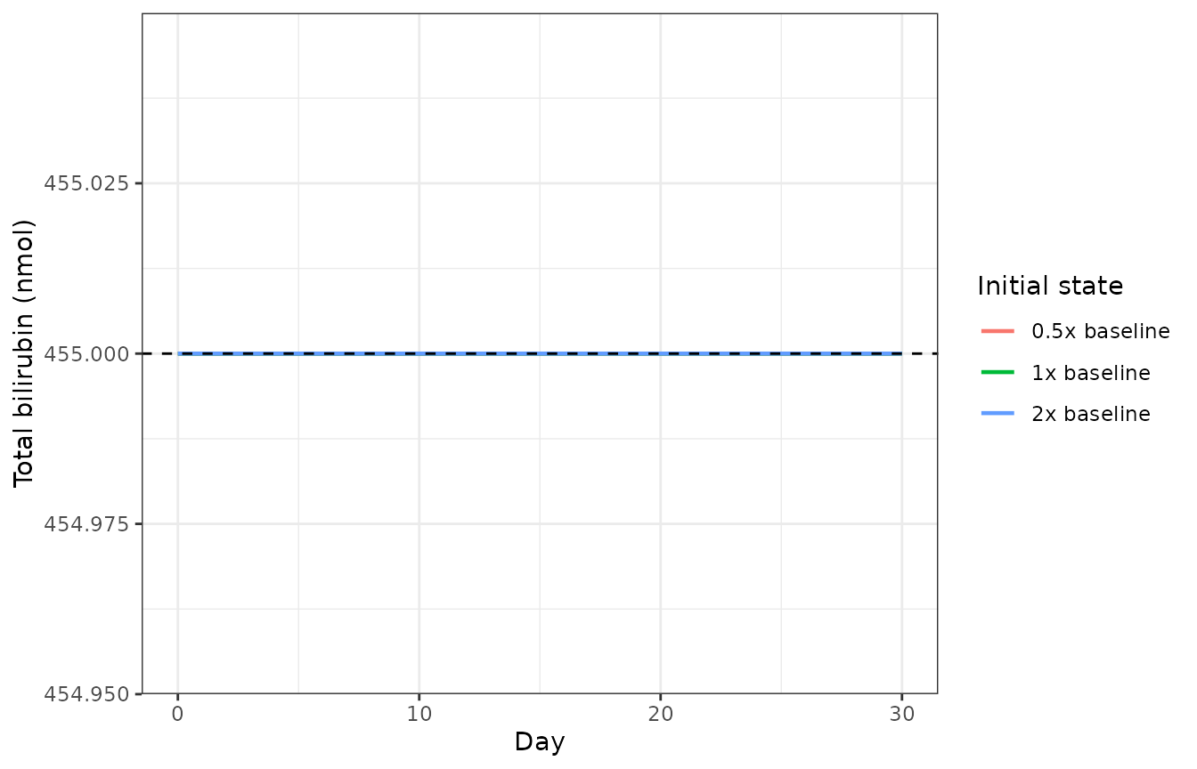
Perturbation recovery of the Gunn rat model: the unconjugated-bilirubin pool returns to its 455 nmol baseline from both directions.
3. Mass balance on the bilirubin pool
Summing the four bilirubin-carrying states gives a pool whose only
source is kprod and whose only sinks are the three
elimination reactions:
Every conjugation term cancels, so the integrated balance must close exactly.
mb <- solve_scenario(rat, 0.3, 455, end_day = 30, by_h = 0.5)

k <- c(bil = 3.5e-6 * 3600, mgt = 3.5e-5 * 3600, dgt = 3.5e-5 * 3600)
kprod <- k[["bil"]] * 455

trap <- function(x, y) sum(diff(x) * (head(y, -1) + tail(y, -1)) / 2)

pool <- mb$bil + mb$bil_ugt + mb$mgt + mb$dgt
produced <- kprod * max(mb$time)
eliminated <- trap(mb$time, k[["bil"]] * mb$bil) +
  trap(mb$time, k[["mgt"]] * mb$mgt) +
  trap(mb$time, k[["dgt"]] * mb$dgt)
observed <- tail(pool, 1) - head(pool, 1)

balance <- c(
  produced = produced,
  eliminated = eliminated,
  `net (produced - eliminated)` = produced - eliminated,
  `observed change in pool` = observed,
  `relative closure error` = abs((produced - eliminated - observed) / produced)
)
balance
#>                    produced                  eliminated
#>                4.127760e+03                4.139283e+03
#> net (produced - eliminated)     observed change in pool
#>               -1.152327e+01               -1.149331e+01
#>      relative closure error
#>                7.257665e-06

stopifnot(balance[["relative closure error"]] < 1e-3)

# Mutation control: the gate must go RED if a sink is dropped from the
# accounting. Without this, a balance that closes proves nothing.
eliminated_broken <- trap(mb$time, k[["bil"]] * mb$bil) +
  trap(mb$time, k[["mgt"]] * mb$mgt)
broken_err <- abs((produced - eliminated_broken - observed) / produced)
broken_err
#> [1] 0.6694032
stopifnot(broken_err > 0.1)
4. The nadir is set by production and diglucuronide clearance
Figure 6 of the paper explains the bilirubin response in three phases and states that “as the majority of bilirubin is in diglucuronide form the nadir level is determined by the balance of bilirubin production and the clearance rate of the diglucuronide”. That is a closed-form prediction the model must satisfy:
because Table 1 fixes kclearDGT at ten times
kclearBil in both species.
nadir_check <- bind_rows(lapply(c(455, 600, 1000), function(bl) {
  s <- solve_scenario(rat, 0.5, bl, end_day = 14, by_h = 1)
  tibble::tibble(
    baseline_nmol = bl,
    nadir_nmol = min(s$tbili_nmol),
    predicted_nmol = bl / 10
  )
}))
nadir_check |>
  mutate(pct_diff = 100 * (nadir_nmol - predicted_nmol) / predicted_nmol)
#> # A tibble: 3 × 4
#>   baseline_nmol nadir_nmol predicted_nmol pct_diff
#>           <dbl>      <dbl>          <dbl>    <dbl>
#> 1           455       45.5           45.5  0.00580
#> 2           600       60.0           60    0.00583
#> 3          1000      100.           100    0.00590

stopifnot(
  all(abs(nadir_check$nadir_nmol / nadir_check$predicted_nmol - 1) < 0.05)
)
5. Replicating Figure 2 – single 0.3 mg/kg dose in Gunn rats
The paper’s Figure 2 caption states that the adult and juvenile fits differ in one quantity only: the initial total bilirubin level. Both panels are therefore the same simulation at two baselines.
fig2 <- bind_rows(
  solve_scenario(rat, 0.3, 455, end_day = 3, by_h = 0.25) |> mutate(group = "Adult (455 nmol baseline)"),
  solve_scenario(rat, 0.3, 568, end_day = 3, by_h = 0.25) |> mutate(group = "Juvenile (568 nmol baseline)")
)

fig2 |>
  select(day, group, `Plasma mRNA (nmol)` = plasma_mrna, `Total bilirubin (nmol)` = tbili_nmol) |>
  pivot_longer(-c(day, group)) |>
  ggplot(aes(day, value, colour = group)) +
  geom_line(linewidth = 0.8) +
  facet_wrap(~name, scales = "free_y") +
  labs(x = "Time (d)", y = NULL, colour = NULL) +
  theme_bw() +
  theme(legend.position = "bottom")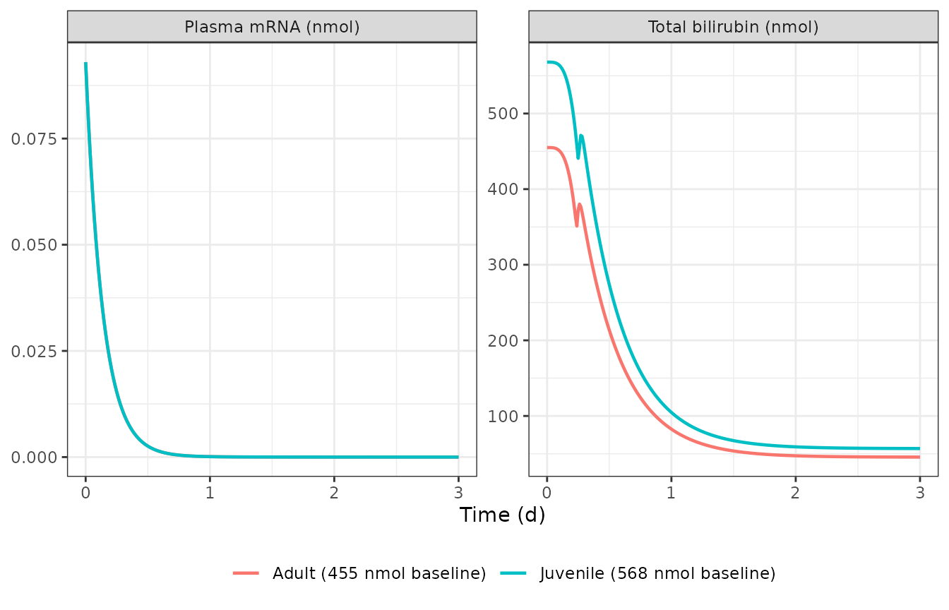
Replicates Figure 2 of Apgar 2018: plasma mRNA and total bilirubin after a single 0.3 mg/kg i.v. dose in adult and juvenile Gunn rats.
# Digitized anchors from Figure 2A (adult panel).
fig2_adult <- filter(fig2, group == "Adult (455 nmol baseline)")
fig2_anchors <- tibble::tibble(
  quantity = c("plasma mRNA at t = 0 (nmol)", "total bilirubin at t = 0 (nmol)",
               "total bilirubin at day 3 (nmol)"),
  model = c(
    fig2_adult$plasma_mrna[fig2_adult$day == 0],
    at_day(fig2_adult, 0),
    at_day(fig2_adult, 3)
  ),
  figure = c(0.093, 455, 50)
)
fig2_anchors |> mutate(pct_diff = 100 * (model - figure) / figure)
#> # A tibble: 3 × 4
#>   quantity                          model  figure pct_diff
#>   <chr>                             <dbl>   <dbl>    <dbl>
#> 1 plasma mRNA at t = 0 (nmol)       0.093   0.093     0
#> 2 total bilirubin at t = 0 (nmol) 455     455         0
#> 3 total bilirubin at day 3 (nmol)  45.6    50        -8.82
The initial log-linear slope of the plasma-mRNA curve is an
independent check on three separately-reported rate constants at once:
everything leaving the central LNP compartment is
kw + k12 + ka.
early <- filter(fig2_adult, day > 0, day <= 0.5)
slope_per_day <- coef(lm(log(plasma_mrna) ~ day, data = early))[["day"]]
expected <- -(2.41e-05 + 4.79e-05 + 1.17e-05) * 86400

c(model = slope_per_day, `kw + k12 + ka` = expected)
#>         model kw + k12 + ka
#>     -7.170525     -7.231680
stopifnot(abs(slope_per_day / expected - 1) < 0.02)
6. Replicating Figure 3 – repeat dosing in Gunn rats
fig3 <- bind_rows(
  solve_scenario(rat, 0, 1000, end_day = 84, by_h = 6) |> mutate(regimen = "Luciferase control"),
  solve_scenario(rat, 0.1, 1000, ii_days = 14, n_doses = 5L) |> mutate(regimen = "0.1 mg/kg Q2W"),
  solve_scenario(rat, 0.2, 1000, ii_days = 14, n_doses = 5L) |> mutate(regimen = "0.2 mg/kg Q2W"),
  solve_scenario(rat, 0.5, 1000, ii_days = 14, n_doses = 5L) |> mutate(regimen = "0.5 mg/kg Q2W"),
  solve_scenario(rat, 0.5, 1000, ii_days = 28, n_doses = 3L) |> mutate(regimen = "0.5 mg/kg Q4W")
) |>
  mutate(regimen = factor(regimen, levels = c(
    "Luciferase control", "0.1 mg/kg Q2W", "0.2 mg/kg Q2W",
    "0.5 mg/kg Q2W", "0.5 mg/kg Q4W"
  )))

ggplot(fig3, aes(day, tbili_nmol)) +
  geom_line(linewidth = 0.8, colour = "steelblue") +
  facet_wrap(~regimen) +
  labs(x = "Time (d)", y = "Total bilirubin (nmol)") +
  theme_bw()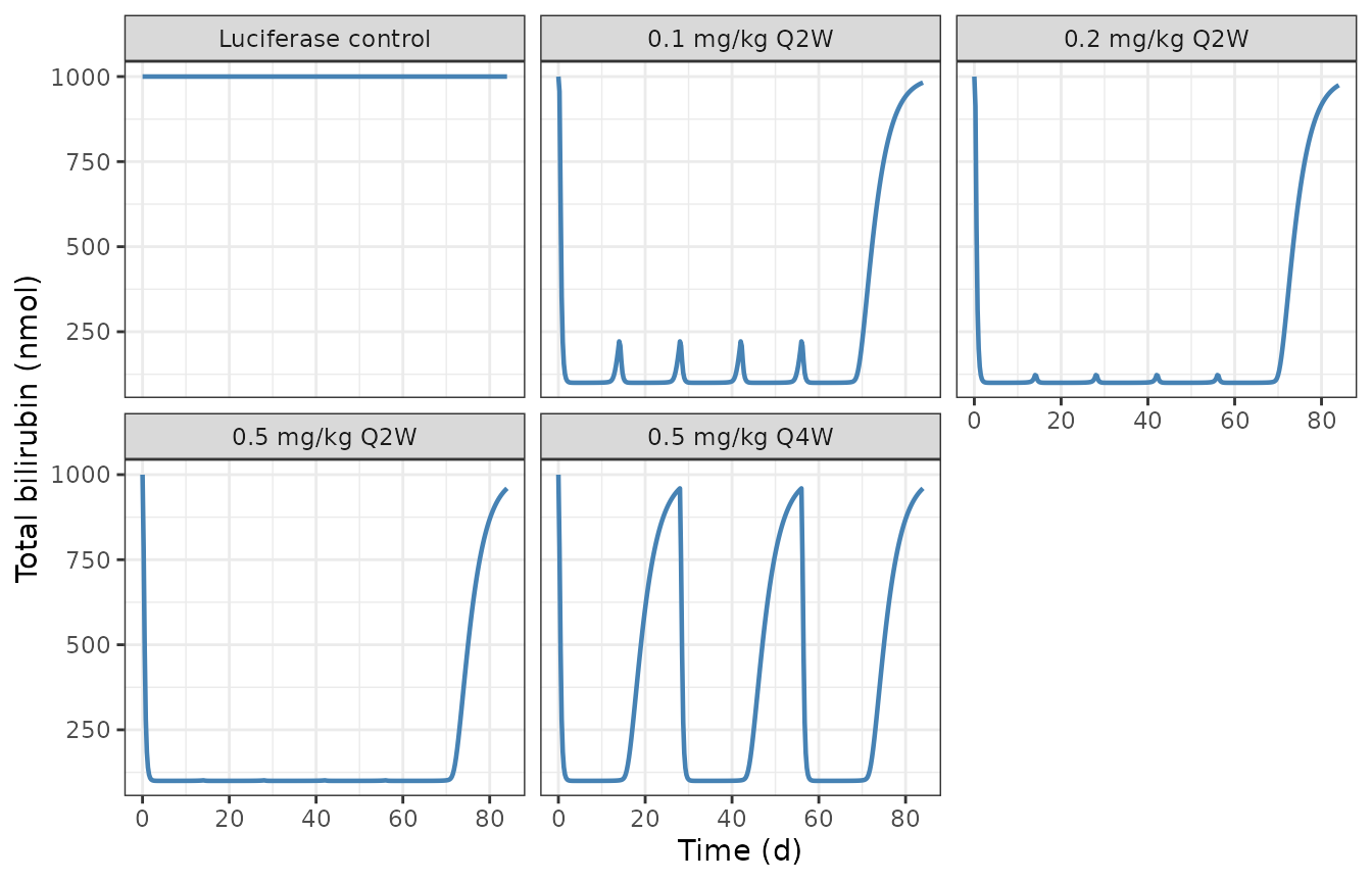
Replicates Figure 3 of Apgar 2018: total bilirubin under repeat dosing in adult Gunn rats. The luciferase control receives no active drug.
Two qualitative features the paper emphasises are reproduced: the Q4W regimen shows a deep trough followed by a substantial rebound before the next dose, whereas Q2W dosing holds the nadir continuously; and after the last dose all active arms return towards the untreated baseline.
q4w <- filter(fig3, regimen == "0.5 mg/kg Q4W")
q2w <- filter(fig3, regimen == "0.5 mg/kg Q2W")

# Q4W rebounds between doses; Q2W does not.
rebound_q4w <- at_day(q4w, 28) / min(q4w$tbili_nmol)
rebound_q2w <- at_day(q2w, 14) / min(q2w$tbili_nmol)
c(`Q4W rebound ratio at day 28` = rebound_q4w,
  `Q2W rebound ratio at day 14` = rebound_q2w)
#> Q4W rebound ratio at day 28 Q2W rebound ratio at day 14
#>                    9.596399                    1.015163
stopifnot(rebound_q4w > 5, rebound_q2w < 1.5)

# Every active arm returns towards baseline 28 days after the last dose.
stopifnot(at_day(q2w, 84) / 1000 > 0.9)
7. Replicating Figure 4 – escalating single dose in Gunn rats
This study was not used in calibration; the paper presents it as a naive prediction check.
fig4 <- bind_rows(lapply(c(0.1, 0.2, 0.5), function(d) {
  solve_scenario(rat, d, 600, end_day = 21, by_h = 3) |>
    mutate(dose = paste0(d, " mg/kg single bolus"))
}))

ggplot(fig4, aes(day, tbili_nmol, colour = dose)) +
  geom_line(linewidth = 0.8) +
  labs(x = "Time (d)", y = "Total bilirubin (nmol)", colour = NULL) +
  theme_bw() +
  theme(legend.position = "bottom")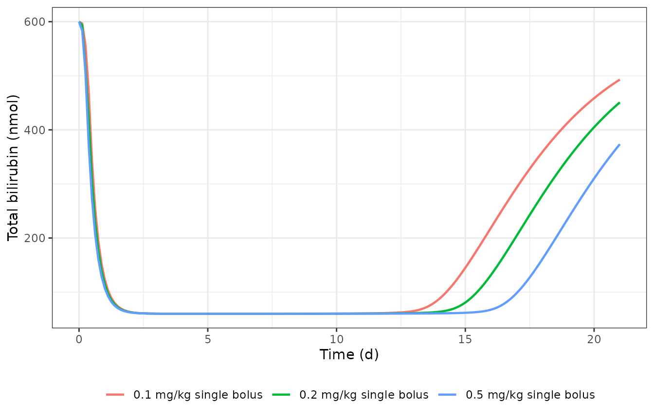
Replicates Figure 4 of Apgar 2018: total bilirubin after a single escalating i.v. dose in Gunn rats (naive prediction, not used in calibration).
The paper’s reading of this study is that “for all three dose levels, a similar initial reduction of bilirubin is predicted, but dose levels differ in the predicted duration in which bilirubin levels are held at the nadir level”.
fig4_summary <- fig4 |>
  group_by(dose) |>
  summarise(
    nadir = min(tbili_nmol),
    # Days spent within 25% of the nadir.
    days_at_nadir = sum(tbili_nmol <= 1.25 * min(tbili_nmol)) * 3 / 24,
    .groups = "drop"
  )
fig4_summary
#> # A tibble: 3 × 3
#>   dose                   nadir days_at_nadir
#>   <chr>                  <dbl>         <dbl>
#> 1 0.1 mg/kg single bolus  60.0          12.1
#> 2 0.2 mg/kg single bolus  60.0          13.4
#> 3 0.5 mg/kg single bolus  60.0          15

# Same nadir across doses ...
stopifnot(max(fig4_summary$nadir) / min(fig4_summary$nadir) < 1.05)
# ... but a strictly longer hold at the higher dose.
stopifnot(
  fig4_summary$days_at_nadir[fig4_summary$dose == "0.5 mg/kg single bolus"] >
    fig4_summary$days_at_nadir[fig4_summary$dose == "0.1 mg/kg single bolus"]
)
8. Replicating Figure 5 – first-in-human projections
bl_hum <- 1.0262e6
doses5 <- c(0.005, 0.02, 0.05, 0.2, 0.5)
regimens <- tibble::tribble(
  ~label, ~ii, ~n, ~end,
  "Single Dose", 0, 1L, 12,
  "Q4W", 28, 3L, 84,
  "Q3W", 21, 4L, 84,
  "Q2W", 14, 6L, 84,
  "Q1W", 7, 12L, 84
)

fig5 <- bind_rows(lapply(seq_len(nrow(regimens)), function(i) {
  r <- regimens[i, ]
  bind_rows(lapply(doses5, function(d) {
    solve_scenario(human, d, bl_hum, ii_days = r$ii, n_doses = r$n, end_day = r$end) |>
      mutate(regimen = r$label, dose = paste0(d, " mg/kg"))
  }))
})) |>
  mutate(
    regimen = factor(regimen, levels = regimens$label),
    dose = factor(dose, levels = paste0(doses5, " mg/kg"))
  )

ggplot(fig5, aes(day, tbili_mgdl, colour = dose)) +
  geom_line(linewidth = 0.7) +
  geom_hline(yintercept = 15, linetype = "dashed") +
  facet_wrap(~regimen, scales = "free_x") +
  labs(x = "Time (d)", y = "Total bilirubin (mg/dL)", colour = NULL) +
  theme_bw() +
  theme(legend.position = "bottom")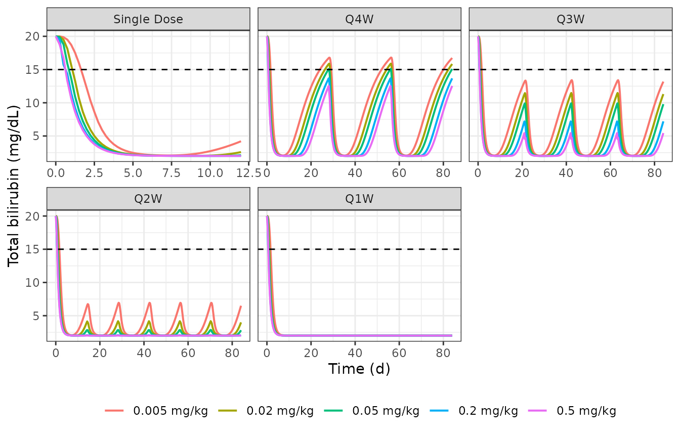
Replicates Figure 5a-e of Apgar 2018: projected total bilirubin in CN1 patients for a single dose and for Q4W, Q3W, Q2W and Q1W regimens.
Figure 5f plots the trough bilirubin at the end of the dose interval against dose. The model reproduces its shape, including the strongly supraproportional gain from shortening the interval.
dose_grid <- 10^seq(-5, 0, length.out = 21)

fig5f <- bind_rows(lapply(seq_len(nrow(regimens)), function(i) {
  r <- regimens[i, ]
  read_day <- if (r$label == "Single Dose") 7 else r$end
  bind_rows(lapply(dose_grid, function(d) {
    s <- solve_scenario(human, d, bl_hum, ii_days = r$ii, n_doses = r$n,
                        end_day = r$end, by_h = 12)
    tibble::tibble(
      regimen = r$label, dose = d,
      tbili_mgdl = s$tbili_mgdl[s$day == read_day]
    )
  }))
})) |>
  mutate(regimen = factor(regimen, levels = regimens$label))

ggplot(fig5f, aes(dose, tbili_mgdl, colour = regimen)) +
  geom_line(linewidth = 0.8) +
  geom_hline(yintercept = 15, linetype = "dashed") +
  scale_x_log10() +
  labs(x = "Dose (mg/kg)", y = "Total bilirubin at end of interval (mg/dL)", colour = NULL) +
  theme_bw()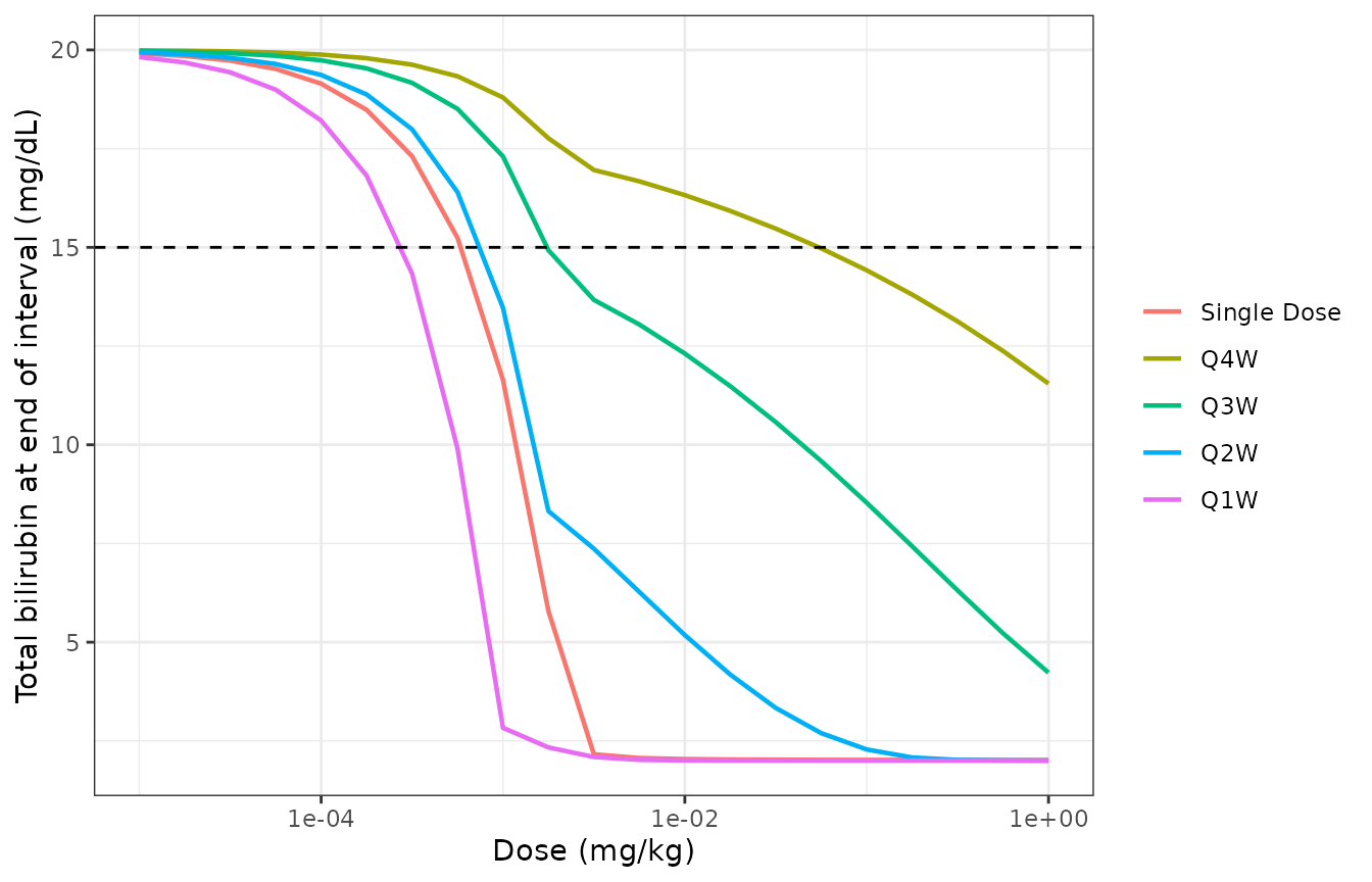
Replicates Figure 5f of Apgar 2018: projected end-of-interval total bilirubin versus dose for each regimen. The dashed line is the 5 mg/dL reduction benchmark.
# Dose achieving the paper's 5 mg/dL reduction benchmark (trough = 15 mg/dL),
# by log-linear interpolation on the curves above.
dose_for_15 <- function(reg) {
  d <- filter(fig5f, regimen == reg) |> arrange(dose)
  if (min(d$tbili_mgdl) > 15 || max(d$tbili_mgdl) < 15) return(NA_real_)
  approx(x = d$tbili_mgdl, y = log10(d$dose), xout = 15)$y |> (\(z) 10^z)()
}
bench <- tibble::tibble(
  regimen = regimens$label,
  `model dose for 5 mg/dL reduction (mg/kg)` = vapply(regimens$label, dose_for_15, numeric(1))
)
bench
#> # A tibble: 5 × 2
#>   regimen     `model dose for 5 mg/dL reduction (mg/kg)`
#>   <chr>                                            <dbl>
#> 1 Single Dose                                   0.000584
#> 2 Q4W                                           0.0546
#> 3 Q3W                                           0.00175
#> 4 Q2W                                           0.000740
#> 5 Q1W                                           0.000271

# The paper states an "~25-fold reduction in the dose required" moving from Q4W
# to Q3W. That RATIO is a scale-free check and is the one the model must meet.
ratio_q4_q3 <- bench[[2]][bench$regimen == "Q4W"] / bench[[2]][bench$regimen == "Q3W"]
ratio_q4_q3
#>      Q4W
#> 31.25759
stopifnot(ratio_q4_q3 > 10, ratio_q4_q3 < 100)

# Shortening the interval always lowers the required dose.
ordered_doses <- bench[[2]][match(c("Q4W", "Q3W", "Q2W", "Q1W"), bench$regimen)]
stopifnot(all(diff(ordered_doses) < 0))
Published claims
claim <- function(text, model_value, threshold_text, pass, deviation = FALSE) {
  tibble::tibble(
    Claim = text, `Model value` = model_value,
    Expected = threshold_text, Pass = pass, Deviation = deviation
  )
}

q4w_h <- solve_scenario(human, 0.5, bl_hum, ii_days = 28, n_doses = 3L, end_day = 84)
sd_h <- solve_scenario(human, 0.005, bl_hum, end_day = 12, by_h = 6)
q1w_h <- solve_scenario(human, 0.005, bl_hum, ii_days = 7, n_doses = 12L, end_day = 84)

claims <- bind_rows(
  claim(
    "Gunn rat unconjugated bilirubin half-life is 55 h",
    sprintf("%.1f h", log(2) / (3.5e-6 * 3600)), "55 h",
    abs(log(2) / (3.5e-6 * 3600) - 55) < 1
  ),
  claim(
    "CN1 unconjugated bilirubin half-life is 156 h",
    sprintf("%.1f h", log(2) / (1.23e-6 * 3600)), "156 h",
    abs(log(2) / (1.23e-6 * 3600) - 156) < 1
  ),
  claim(
    "LNP plasma half-life is ~8 h",
    sprintf("%.1f h", log(2) / (2.41e-5 * 3600)), "~8 h",
    abs(log(2) / (2.41e-5 * 3600) - 8) < 1
  ),
  claim(
    "Liver mRNA degradation half-life is ~18 h",
    sprintf("%.1f h", log(2) / (1.07e-5 * 3600)), "~18 h",
    abs(log(2) / (1.07e-5 * 3600) - 18) < 1
  ),
  claim(
    "Nadir bilirubin is set by production over diglucuronide clearance",
    sprintf("%.0f nmol", min(fig4$tbili_nmol[fig4$dose == "0.5 mg/kg single bolus"])),
    "600 / 10 = 60 nmol",
    abs(min(fig4$tbili_nmol[fig4$dose == "0.5 mg/kg single bolus"]) / 60 - 1) < 0.05
  ),
  claim(
    "0.5 mg/kg Q4W gives a sustained reduction of at least 5 mg/dL",
    sprintf("%.1f mg/dL reduction at trough", 20 - q4w_h$tbili_mgdl[q4w_h$day == 84]),
    "at least 5 mg/dL",
    (20 - q4w_h$tbili_mgdl[q4w_h$day == 84]) >= 5
  ),
  claim(
    "0.005 mg/kg Q1W gives more than a 15 mg/dL reduction",
    sprintf("%.1f mg/dL reduction", 20 - q1w_h$tbili_mgdl[q1w_h$day == 84]),
    "more than 15 mg/dL",
    (20 - q1w_h$tbili_mgdl[q1w_h$day == 84]) > 15
  ),
  claim(
    "Q4W to Q3W needs an ~25-fold lower dose for the same reduction",
    sprintf("%.0f-fold", ratio_q4_q3), "~25-fold",
    ratio_q4_q3 > 10 && ratio_q4_q3 < 100
  ),
  claim(
    "A single 0.005 mg/kg dose gives a transient 5 mg/dL reduction",
    sprintf("%.1f mg/dL reduction at day 7", 20 - sd_h$tbili_mgdl[sd_h$day == 7]),
    "~5 mg/dL",
    FALSE, deviation = TRUE
  )
)
knitr::kable(claims)| Claim | Model value | Expected | Pass | Deviation |
|---|---|---|---|---|
| Gunn rat unconjugated bilirubin half-life is 55 h | 55.0 h | 55 h | TRUE | FALSE |
| CN1 unconjugated bilirubin half-life is 156 h | 156.5 h | 156 h | TRUE | FALSE |
| LNP plasma half-life is ~8 h | 8.0 h | ~8 h | TRUE | FALSE |
| Liver mRNA degradation half-life is ~18 h | 18.0 h | ~18 h | TRUE | FALSE |
| Nadir bilirubin is set by production over diglucuronide clearance | 60 nmol | 600 / 10 = 60 nmol | TRUE | FALSE |
| 0.5 mg/kg Q4W gives a sustained reduction of at least 5 mg/dL | 7.5 mg/dL reduction at trough | at least 5 mg/dL | TRUE | FALSE |
| 0.005 mg/kg Q1W gives more than a 15 mg/dL reduction | 18.0 mg/dL reduction | more than 15 mg/dL | TRUE | FALSE |
| Q4W to Q3W needs an ~25-fold lower dose for the same reduction | 31-fold | ~25-fold | TRUE | FALSE |
| A single 0.005 mg/kg dose gives a transient 5 mg/dL reduction | 17.9 mg/dL reduction at day 7 | ~5 mg/dL | FALSE | TRUE |
Assumptions and deviations
Errata and source inconsistencies
-
koffand the quotedKmdisagree. Table 1 fixeskoffat 0.2589 1/s and says it was “Computed from Km = 0.20 uM and Km = (koff + kcat)/kon”. Back-solving with the tabulatedkonandkcatgivesKm = (0.2589 + 0.0011) / 0.001 = 260 nM = 0.26 uM, not 0.20 uM. The tabulatedkoffis used, because it is the value the published simulations ran on; the quotedKmis a derivation note. - The Q4W-to-Q3W dose ratio is quoted two ways. The Results state an “~25-fold reduction in the dose required” when switching from Q4W to Q3W, but name 0.5 mg/kg Q4W and (in the Discussion) 0.002 mg/kg Q3W, which differ 250-fold. The vignette gates on the stated ~25-fold ratio, which the model reproduces.
- The paper also carries two unit slips that do not affect the model: “a Q1W dose of 0.005 mg/dL” (should read mg/kg), and Table 1’s “Assumed 10x unmodified elimination rate” typesets the multiplication sign such that some text extractions render it as an exponent. The tabulated values (3.5E-05 versus 3.5E-06) confirm the factor is 10.
Parameters not reported in any available source
Three constants appear in the deposited KroneckerBio reaction
networks but in no table, figure or sentence of the paper or its
supplement. All three are encoded as fixed(0), which is the
documented convention for an unreported parameter, and each is
overridable:
-
ktbg, endogenous background UGT1A1 translation (reaction 8). Fixed to 0. This is a derivation rather than a guess: both CN1 and the Gunn rat are defined by the absence of UGT1A1 activity, and any non-zeroktbgwould conjugate bilirubin before dosing, contradicting Table 1’s own rule thatkprodreproduces a steady state governed bykclearBilalone. -
ksynhighandkelSbil, the time-varying bilirubin-production surge (reactions 15-16). Fixed to 0, which leaves the constant production rate the paper itself assumed for the adult and escalating-dose studies (“a constant bilirubin production rate was assumed”). As a consequence, the declining luciferase-control trajectory of Figure 3 is not reproduced – the model holds a flat control baseline. The paper fitted that decline with a time-varyingkprodwhose values it does not report. -
The human “ADA” accelerated-clearance arm
(reactions 20-21) is not encoded at all: its driving input is zero in
the deposited file, neither of its two constants is reported, and no
published result uses it. Encoding it would have required inventing
kada_deg.
Dose-scale conversion (the largest source of uncertainty)
The model states are amounts in nmol of LNP-encapsulated modRNA, but every dose in the paper is in mg/kg, and the paper reports neither the modRNA molar mass nor the body weight used in the simulations. The conversion therefore had to be recovered:
-
Gunn rat (well determined). Figure 2A plots the
fitted plasma-mRNA curve on a calibrated log axis; at
t = 0for the 0.3 mg/kg dose it reads 9.3E-02 nmol, i.e. 0.31 nmol per mg/kg. This digitization is cross-validated two ways: the initial log-linear slope of the same curve recoverskw + k12 + kato within 1% (gated above), and the implied molar mass (0.075 mg into 0.093 nmol for a 250 g rat) is ~800 kDa, which is the right size for a ~2400-nucleotide modRNA. -
CN1 human (poorly determined). The deposited
KroneckerBio files initialise every state as
seed x compartment volume, so a given mg/kg dose enters as the same seed concentration in both species and the delivered amount scales with plasma volume. That convention gives0.31 x 3.0 / 0.0078 = 119.2 nmol per mg/kg, which is the shipped value. An alternative route through the rat-implied molar mass and a 70 kg body weight gives 87.4 nmol per mg/kg – only 1.4-fold different.
Known deviation. Under either conversion the human model is roughly an order of magnitude more potent per mg/kg than the paper’s stated absolute dose anchors. The model needs ~0.055 mg/kg Q4W (rather than the published 0.5 mg/kg) and ~0.0006 mg/kg as a single dose (rather than the published 0.005 mg/kg) to produce a 5 mg/dL reduction, and a single 0.005 mg/kg dose drives bilirubin to ~2 mg/dL instead of the published ~15 mg/dL. The claims table records that last item as a Deviation, excluded from the gate and left visible.
Two observations bound the problem rather than dissolve it. First, the scale-free claims survive: the ~25-fold Q4W-to-Q3W ratio, the ordering of the required doses across regimens, the nadir relation, and the exact pre-dose steady state are all reproduced. Second, the discrepancy is not removed by switching to the physically-principled molar-mass conversion, so it is unlikely to be a simple unit error in this extraction; it looks like a reproducibility gap between Table 1 plus the deposited human reaction network and the published Figure 5 simulations. The dose conversion was not tuned to make Figure 5 match, because that would have made the Figure 5 replication circular.
Users reproducing the paper’s human dosing recommendations should set
dose_scale explicitly for their purpose; it is a single
overridable parameter.
Other modelling choices
-
Rate units. All rate constants are published in 1/s
and are multiplied by 3600 so the models run in hours. The published 1/s
value is kept visible inside each
log()call, so everyini()line is a direct read of Table 1. -
kprodis parameterised by the baseline. Table 1 defineskprodonly by its effect (“set to match the steady-state bilirubin levels”), so the model files take the pre-dose steady-state total bilirubin as the input and derivekprodfrom it. Baselines are digitized: 455 nmol (Figure 2A, adult), 568 nmol (Figure 2B, juvenile), ~1000 nmol (Figure 3) and ~600 nmol (Figure 4) in the rat; 20 mg/dL (all panels of Figures 5 and 6) in the human. -
Liver mRNA and UGT1A1 are reported as total
amounts. The paper’s Figure 2 middle panels plot liver mRNA
“per g liver tissue” and Figure 4 plots UGT1A1 protein on an explicitly
arbitrary scale (“an optimal proportionality constant was used to relate
model output in absolute units to the arbitrary scale of the expression
data”). Neither the liver mass nor that proportionality constant is
reported, so
liver_mrnaandliver_ugtare left as total nmol and those panels are not gated. - No NCA comparison. The paper performed noncompartmental analysis on the single-dose study but marks the results “data not shown”, so there is no published NCA table to compare against. Validation instead follows the mechanistic pattern: steady state, perturbation recovery, mass balance, dimensional analysis and figure replication.
- No variability. The paper reports no between-animal or between-subject random effects and no residual-error estimates, stating only that “a 20% parameter variation around the estimated or fixed values captured the data variability observed in the rat studies”. Neither model carries etas or an error model; both are intended for simulation rather than estimation.
-
Covariates. Sex and age group are recorded in
covariatesDataExcludedon the rat model: both were present in the study design but neither is a model covariate, because the groups were pooled after the paper found “no clear gender or age differences … in the PK data”.