Sparsentan (Wada 2023)

Model and source

• Citation: Wada R, Kleijn HJ, Zhang L, Chen S-C. Population pharmacokinetic analysis of sparsentan in healthy volunteers and patients with focal segmental glomerulosclerosis. CPT Pharmacometrics Syst Pharmacol. 2023;12(8):1080-1092. doi:10.1002/psp4.12996
• Description: Two-compartment population PK model with lagged first-order absorption for oral sparsentan (a single-molecule dual endothelin / angiotensin II receptor antagonist, DEARA) pooled over nine phase I-III studies in 446 subjects: 236 healthy volunteers, 16 subjects with hepatic impairment, and 194 patients with primary or genetic focal segmental glomerulosclerosis (FSGS). Apparent oral clearance carries a first-order CYP3A auto-induction term that steps CL/F from 3.88 L/h on the first dosing day to 5.11 L/h thereafter (induction half-life fixed at 0.001 day, i.e. effectively instantaneous), multiplied by power effects of alkaline phosphatase and creatinine clearance and by log-additive effects of male sex and of moderate / strong CYP3A4 inhibitor coadministration. Relative bioavailability is a power function of dose clamped at 200 mg, producing less-than-dose-proportional exposure (Frel = 1.41, 1.00, 0.71 at 200, 400, 800 mg). Race shifts the apparent central volume, and formulation (whole tablet or crushed tablet against the capsule reference) shifts both the absorption rate constant and the absorption lag time. Residual error is combined proportional plus additive, with the additive SD fixed at the 2 ng/mL assay lower limit of quantitation.
• Article: https://doi.org/10.1002/psp4.12996
• Supplement (Tables S1-S4, Figures S1-S3): https://doi.org/10.1002/psp4.12996 (Supporting Information; Table S3 prints the final-model equations verbatim and is the primary structural source for this extraction)

Sparsentan is a single-molecule dual endothelin / angiotensin II receptor antagonist (DEARA) developed for focal segmental glomerulosclerosis (FSGS) and IgA nephropathy. Wada 2023 pooled nine phase I-III studies into one population PK analysis, and this vignette reproduces its published typical-value parameters, covariate influences, and steady-state exposures from the packaged model.

Population

The analysis dataset held 10,957 plasma sparsentan concentrations from 446 subjects across nine studies (Wada 2023 Table S1): 236 healthy volunteers in six phase I studies, 16 subjects with mild or moderate hepatic impairment (plus 12 matched healthy volunteers) in one phase I study, and 194 patients with primary or genetic FSGS in the phase II DUET and phase III DUPLEX trials.

Baseline characteristics (Wada 2023 Table 1, overall column): median age 40 years (range 8-74), median body weight 78.6 kg (range 21.1-154.0), 33.2% female, 67.5% White / 23.5% Black or African American / 6.1% Asian / 0.7% Multiple / 2.2% Other. Median creatinine clearance was 112 mL/min (range 26-361) and median alkaline phosphatase 68 U/L (range 25-269). Renal function was normal in 74.2%, mildly impaired in 13.5%, moderately impaired in 11.9%, and severely impaired in only 2 subjects (0.4%) - too few for conclusions about severe renal impairment. Doses ranged from single 50-1600 mg administrations in phase I to 200-800 mg once daily in DUET and DUPLEX. Bioanalysis was validated LC-MS/MS over 2-4000 ng/mL with a 2 ng/mL LLOQ; all BLQ samples were excluded.

The same information is available programmatically via the model’s population metadata (readModelDb("Wada_2023_sparsentan")()$population).

Source trace

The per-parameter origin is recorded as an in-file comment next to each ini() entry in inst/modeldb/specificDrugs/Wada_2023_sparsentan.R. The table below collects them in one place for review. All reference-subject values are for a White female receiving a 400 mg capsule, no CYP3A4 inhibitor, CrCL 112 mL/min, ALKP 68 U/L (Wada 2023 Table 2 footnote b).

Equation / parameter	Value	Source location
Structural model: 2-compartment, first-order absorption + lag time	n/a	Abstract; Results “Base model”; Table S3
lcl (CL/F pre-induction)	3.88 L/h	Table 2 “CL/F (L/h)”, RSE 4.6%
lcl_time (auto-induction increment on CL/F)	1.23 L/h	Table 2 “Induction change in CL (L/h)”, RSE 13.6%
lkdes (induction onset rate)	693.147 /day, fixed	Table 2 “Induction t 1/2 (day)” = 0.001 fixed; log(2)/0.001
Induction equation CL(t) = CL0 + dCL*(1 - exp(-k*Day))	n/a	Methods “Development of the population PK model”; Table S3
lvc (Vc/F)	49.3 L	Table 2 “V c / F (L)”, RSE 4.3%
lq (Q/F)	2.03 L/h	Table 2 “Q / F (L/h)”, RSE 12.0%
lvp (Vp/F)	12.1 L	Table 2 “V p / F (L)”, RSE 10.5%
lka (Ka, capsule)	0.740 /h	Table 2 “K a (1/h)”, RSE 6.9%
ltlag (Tlag, capsule)	0.32 h	Table 2 “T lag (h)”, RSE 4.0%
e_dose_fdepot (dose on Frel)	-0.495	Table 2 “Dose on F rel”, RSE 5.1%; Table 2 note; Table S3
Frel = (max(DOSE,200)/400)^-0.495	n/a	Table 2 note; Table S3
e_alp_cl	-0.208	Table 2 “Effect on CL / ALKP”, RSE 27.5%; Table S3 (ALKP/68)^-0.208
e_crcl_cl	0.222	Table 2 “Effect on CL / CrCL”, RSE 26.5%; Table S3 (CrCL/112)^0.222
e_sexf_cl (male effect)	0.139	Table 2 “Effect on CL / Male”, RSE 32.8%; Table S3 x exp[0.139] if Male
e_conmed_cyp3a4_inh_mod_cl	-0.273	Table 2 “Effect on CL / Moderate CYP3A4”, RSE 18.8%
e_conmed_cyp3a4_inh_strong_cl	-1.069	Table 2 “Effect on CL / Strong CYP3A4”, RSE 10.0%
e_race_black_vc	0.309	Table 2 “Effect on Vc / Black or African American”, RSE 18.4%
e_race_asian_vc	0.265	Table 2 “Effect on Vc / Asian”, RSE 48.4%
e_form_tablet_ka	-0.306	Table 2 “Effect on K a / Tablet”, RSE 34.8%
e_form_crushed_tablet_ka	0.080	Table 2 “Effect on K a / Crushed tablet”, RSE 159.1%
e_form_tablet_tlag	-0.269	Table 2 “Effect on T lag / Tablet”, RSE 29.1%
e_form_crushed_tablet_tlag	-1.175	Table 2 “Effect on T lag / Crushed tablet”, RSE 28.7%
etalcl (variance)	0.156	Table 2 “Variance CL”, RSE 8.7% (IIV 39.5% = sqrt(0.156))
etalvc (variance)	0.234	Table 2 “Variance V c”, RSE 11.3% (IIV 48.4% = sqrt(0.234))
etalka (variance)	0.474	Table 2 “Variance K a”, RSE 10.2% (IIV 68.9% = sqrt(0.474))
propSd	0.365	Table 2 “SD of proportional error”, RSE 1.9%
addSd	2 ng/mL = 0.002 ug/mL, fixed	Table 2 “SD of additive error (ng/mL)”, fixed at the LLOQ
Covariate model form (log-domain; median-scaled continuous, most-frequent-level reference categorical)	n/a	Methods “Development of the population PK model”; Table 1
Reference subject definition	n/a	Table 2 footnote b

Validation targets used below:

Target	Published value	Source
CL/F, reference subject, first dose	3.88 L/h	Table 2; Results “Final model”
CL/F, reference subject, steady state	5.12 L/h	Table 2 (derived); Results “Final model”
CL/F, 800 mg, single dose / steady state	5.47 / 7.21 L/h	Table 2 “800 mg dose” derived rows
Vc/F, Vp/F at 800 mg	69.5 / 17.0 L	Table 2 “800 mg dose” derived rows
Terminal half-life at steady state	9.6 h	Table 2 “T 1/2 (h) (derived)”
Frel at 200 / 400 / 800 mg	1.41 / 1.00 / 0.71	Results “Final model”
Typical FSGS CL/F, Vc/F, Tlag, Ka	7.5 L/h, 69 L, 0.24 h, 0.54 /h	Table 3
Table 3 covariate influences	see table	Table 3
Steady-state AUC, combined high-exposure covariates	193 ug/mL*h	Discussion

Virtual cohort

Original observed data are not publicly available. Two kinds of cohort are built below.

1. Typical-value cohorts (one subject per covariate setting, IIV switched off with omega = NA) to reproduce the published point estimates in Tables 2 and 3 and the formulation comparison of Figure 3.
2. Stochastic cohorts (150 subjects per arm, well under the 200/arm cap) for the VPC-style figures that mirror Figure 1.

# Canonical covariate columns required by the model. Every record - dose and
# observation alike - carries all of them.
COV_DEFAULTS <- list(
  DOSE                     = 400,
  ALP                      = 68,     # overall cohort median (Table 1)
  CRCL                     = 112,    # overall cohort median (Table 1)
  SEXF                     = 1,      # reference subject is female (Table 2 fn b)
  RACE_BLACK               = 0,      # reference race is White
  RACE_ASIAN               = 0,
  FORM_TABLET              = 0,      # reference formulation is the capsule
  FORM_CRUSHED_TABLET      = 0,
  CONMED_CYP3A4_INH_MOD    = 0,
  CONMED_CYP3A4_INH_STRONG = 0
)

#' Build one arm as a plain data frame of dose + observation records.
#'
#' Covariates are attached to the materialised data frame (never assigned onto
#' an rxEt object, where rxode2 silently drops them). Observation rows use the
#' ODE state name `central`; rxode2 returns the algebraic observable `Cc` and
#' every derived quantity (cl, vc, frel, ...) as output columns.
make_arm <- function(arm, n, dose, obs_times, dose_times = 0,
                     id_offset = 0L, covariates = list(), per_id = NULL) {
  cov_vals <- utils::modifyList(COV_DEFAULTS, c(list(DOSE = dose), covariates))
  ids <- id_offset + seq_len(n)

  doses <- tidyr::expand_grid(id = ids, time = dose_times) |>
    dplyr::mutate(amt = dose, evid = 1L, cmt = "depot")
  obs <- tidyr::expand_grid(id = ids, time = obs_times) |>
    dplyr::mutate(amt = NA_real_, evid = 0L, cmt = "central")

  out <- dplyr::bind_rows(doses, obs) |>
    dplyr::arrange(id, time, dplyr::desc(evid)) |>
    dplyr::mutate(arm = arm)
  for (nm in names(cov_vals)) out[[nm]] <- cov_vals[[nm]]

  # Optional per-subject covariate overrides (used for the stochastic arms).
  if (!is.null(per_id)) {
    out <- out |>
      dplyr::select(-dplyr::any_of(setdiff(names(per_id), "id"))) |>
      dplyr::left_join(per_id, by = "id")
  }
  out
}

mod <- readModelDb("Wada_2023_sparsentan")

Reproducing the published typical-value parameters (Tables 2 and 3)

Because the model computes cl, vc, q, vp, ka, tlag and frel inside model(), rxSolve() returns each of them as an output column. Reading them back is therefore an end-to-end check of the packaged model rather than a re-implementation of the paper’s equations. Apparent parameters are recovered as CL/F = cl / frel, Vc/F = vc / frel, and so on.

Note that time = 0 is the first dose, so the whole-day index Day = floor(time / 24) is 0 throughout the first dosing day (pre-induction CL/F) and >= 1 from the second dose onward (fully induced CL/F).

# One subject per covariate setting, dosed QD for 14 days so that both the
# first-dose (Day 0) and the fully-induced (Day >= 1) clearance are observed.
qd_doses <- seq(0, 13 * 24, by = 24)

param_arms <- dplyr::bind_rows(
  # Reference subject (Table 2 footnote b): White female, 400 mg capsule.
  make_arm("Reference, 400 mg capsule", 1, 400,
           obs_times = c(4, 12 * 24 + 4), dose_times = qd_doses,
           id_offset = 0L),
  # Same reference subject at 800 mg, to check the Table 2 "800 mg dose" rows.
  make_arm("Reference, 800 mg capsule", 1, 800,
           obs_times = c(4, 12 * 24 + 4), dose_times = qd_doses,
           id_offset = 10L),
  # 200 mg, to check Frel = 1.41.
  make_arm("Reference, 200 mg capsule", 1, 200,
           obs_times = c(4, 12 * 24 + 4), dose_times = qd_doses,
           id_offset = 20L),
  # Typical FSGS subject (Table 3): White male, 800 mg tablet, ALKP 73,
  # CrCL 78, no moderate or strong CYP3A4 inhibitor.
  make_arm("Typical FSGS, 800 mg tablet", 1, 800,
           obs_times = c(4, 12 * 24 + 4), dose_times = qd_doses,
           id_offset = 30L,
           covariates = list(SEXF = 0, ALP = 73, CRCL = 78, FORM_TABLET = 1))
)

sim_params <- rxode2::rxSolve(
  mod, events = param_arms, omega = NA, keep = "arm"
) |>
  as.data.frame()
#> ℹ parameter labels from comments will be replaced by 'label()'
#> Warning: multi-subject simulation without without 'omega'

# Day 0 = pre-induction; the later sample is fully induced.
published_params <- tibble::tribble(
  ~arm,                          ~quantity,             ~Published,
  "Reference, 400 mg capsule",   "CL/F, first dose (L/h)",   3.88,
  "Reference, 400 mg capsule",   "CL/F, steady state (L/h)", 5.12,
  "Reference, 400 mg capsule",   "Vc/F (L)",                49.3,
  "Reference, 400 mg capsule",   "Vp/F (L)",                12.1,
  "Reference, 400 mg capsule",   "Q/F (L/h)",                2.03,
  "Reference, 400 mg capsule",   "Ka (1/h)",                 0.740,
  "Reference, 400 mg capsule",   "Tlag (h)",                 0.32,
  "Reference, 400 mg capsule",   "Frel",                     1.00,
  "Reference, 800 mg capsule",   "CL/F, first dose (L/h)",   5.47,
  "Reference, 800 mg capsule",   "CL/F, steady state (L/h)", 7.21,
  "Reference, 800 mg capsule",   "Vc/F (L)",                69.5,
  "Reference, 800 mg capsule",   "Vp/F (L)",                17.0,
  "Reference, 800 mg capsule",   "Frel",                     0.71,
  "Reference, 200 mg capsule",   "Frel",                     1.41,
  "Typical FSGS, 800 mg tablet", "CL/F, steady state (L/h)", 7.5,
  "Typical FSGS, 800 mg tablet", "Vc/F (L)",                69,
  "Typical FSGS, 800 mg tablet", "Ka (1/h)",                 0.54,
  "Typical FSGS, 800 mg tablet", "Tlag (h)",                 0.24
)

derived <- sim_params |>
  dplyr::mutate(phase = ifelse(time < 24, "first dose", "steady state")) |>
  dplyr::group_by(arm, phase) |>
  dplyr::slice(1) |>
  dplyr::ungroup() |>
  dplyr::transmute(
    arm, phase,
    `CL/F (L/h)` = cl / frel,
    `Vc/F (L)`   = vc / frel,
    `Vp/F (L)`   = vp / frel,
    `Q/F (L/h)`  = q  / frel,
    `Ka (1/h)`   = ka,
    `Tlag (h)`   = tlag,
    Frel         = frel
  ) |>
  tidyr::pivot_longer(-c(arm, phase), names_to = "quantity",
                      values_to = "Simulated") |>
  dplyr::mutate(
    quantity = dplyr::case_when(
      quantity == "CL/F (L/h)" & phase == "first dose"   ~ "CL/F, first dose (L/h)",
      quantity == "CL/F (L/h)" & phase == "steady state" ~ "CL/F, steady state (L/h)",
      TRUE ~ quantity
    )
  ) |>
  dplyr::filter(!(quantity %in% c("Vc/F (L)", "Vp/F (L)", "Q/F (L/h)",
                                  "Ka (1/h)", "Tlag (h)", "Frel") &
                    phase == "first dose")) |>
  dplyr::select(arm, quantity, Simulated)

comparison <- published_params |>
  dplyr::left_join(derived, by = c("arm", "quantity"))

# Guard: every published target must have found its simulated counterpart. A
# label typo in either frame would silently drop to NA and render a
# plausible-looking table with missing rows.
stopifnot(!anyNA(comparison$Simulated))

comparison |>
  dplyr::mutate(
    `% diff` = round(100 * (Simulated - Published) / Published, 1),
    Simulated = signif(Simulated, 4)
  ) |>
  dplyr::rename("Arm" = arm, "Quantity" = quantity) |>
  knitr::kable(
    caption = paste(
      "Packaged-model typical values against Wada 2023 Tables 2 and 3.",
      "All published values are reproduced within rounding."
    ),
    align = c("l", "l", "r", "r", "r")
  )

Packaged-model typical values against Wada 2023 Tables 2 and 3. All published values are reproduced within rounding.

Arm	Quantity	Published	Simulated	% diff
Reference, 400 mg capsule	CL/F, first dose (L/h)	3.88	3.8800	0.0
Reference, 400 mg capsule	CL/F, steady state (L/h)	5.12	5.1100	-0.2
Reference, 400 mg capsule	Vc/F (L)	49.30	49.3000	0.0
Reference, 400 mg capsule	Vp/F (L)	12.10	12.1000	0.0
Reference, 400 mg capsule	Q/F (L/h)	2.03	2.0300	0.0
Reference, 400 mg capsule	Ka (1/h)	0.74	0.7400	0.0
Reference, 400 mg capsule	Tlag (h)	0.32	0.3200	0.0
Reference, 400 mg capsule	Frel	1.00	1.0000	0.0
Reference, 800 mg capsule	CL/F, first dose (L/h)	5.47	5.4680	0.0
Reference, 800 mg capsule	CL/F, steady state (L/h)	7.21	7.2020	-0.1
Reference, 800 mg capsule	Vc/F (L)	69.50	69.4800	0.0
Reference, 800 mg capsule	Vp/F (L)	17.00	17.0500	0.3
Reference, 800 mg capsule	Frel	0.71	0.7096	-0.1
Reference, 200 mg capsule	Frel	1.41	1.4090	0.0
Typical FSGS, 800 mg tablet	CL/F, steady state (L/h)	7.50	7.5250	0.3
Typical FSGS, 800 mg tablet	Vc/F (L)	69.00	69.4800	0.7
Typical FSGS, 800 mg tablet	Ka (1/h)	0.54	0.5449	0.9
Typical FSGS, 800 mg tablet	Tlag (h)	0.24	0.2445	1.9

Auto-induction step in apparent clearance

# Replicates the Results "Final model" statement that CL/F rises from
# 3.88 L/h after a single 400 mg dose to 5.12 L/h at steady state.
induction_arm <- make_arm(
  "Reference, 400 mg capsule QD", 1, 400,
  obs_times = seq(0, 4 * 24, by = 1), dose_times = seq(0, 3 * 24, by = 24)
)

rxode2::rxSolve(mod, events = induction_arm, omega = NA) |>
  as.data.frame() |>
  dplyr::mutate(`CL/F (L/h)` = cl / frel) |>
  ggplot(aes(time / 24, `CL/F (L/h)`)) +
  geom_step(direction = "hv", linewidth = 0.8) +
  geom_hline(yintercept = c(3.88, 5.12), linetype = "dashed",
             colour = "grey40") +
  annotate("text", x = 3.3, y = 3.88, vjust = -0.6, size = 3,
           label = "published 3.88 L/h (first dose)") +
  annotate("text", x = 3.3, y = 5.12, vjust = 1.6, size = 3,
           label = "published 5.12 L/h (steady state)") +
  scale_x_continuous(breaks = 0:4) +
  labs(x = "Days since first dose", y = "CL/F (L/h)",
       title = "CYP3A auto-induction step in apparent clearance",
       caption = paste(
         "Reproduces Wada 2023 Results 'Final model'. The induction half-life",
         "is fixed at 0.001 day, so the rise is a step between the first and",
         "second dose."))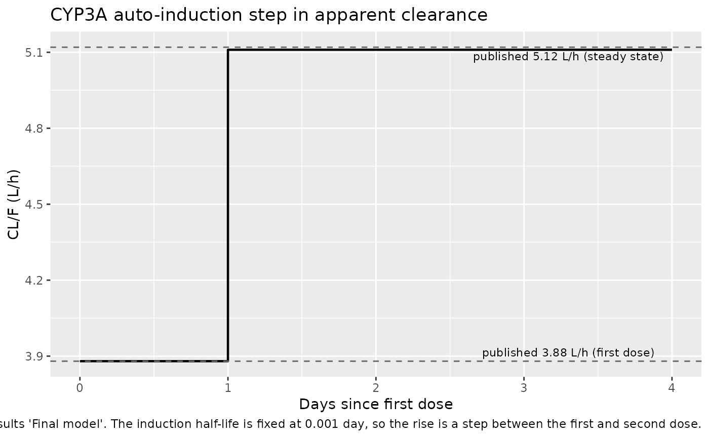

Table 3 covariate influences

# Each row of Wada 2023 Table 3 varies one covariate from the typical FSGS
# subject (White male, 800 mg tablet, ALKP 73 U/L, CrCL 78 mL/min, no
# moderate or strong CYP3A4 inhibitor).
FSGS_TYPICAL <- list(SEXF = 0, ALP = 73, CRCL = 78, FORM_TABLET = 1)

t3_settings <- list(
  list(lbl = "Typical (reference)",            cov = list()),
  list(lbl = "ALKP 40 U/L (5th pct)",          cov = list(ALP = 40)),
  list(lbl = "ALKP 140 U/L (95th pct)",        cov = list(ALP = 140)),
  list(lbl = "CrCL 41 mL/min (5th pct)",       cov = list(CRCL = 41)),
  list(lbl = "CrCL 164 mL/min (95th pct)",     cov = list(CRCL = 164)),
  list(lbl = "Female",                         cov = list(SEXF = 1)),
  list(lbl = "Moderate CYP3A4 inhibitor",      cov = list(CONMED_CYP3A4_INH_MOD = 1)),
  list(lbl = "Strong CYP3A4 inhibitor",        cov = list(CONMED_CYP3A4_INH_STRONG = 1)),
  list(lbl = "Black or African American",      cov = list(RACE_BLACK = 1)),
  list(lbl = "Asian",                          cov = list(RACE_ASIAN = 1)),
  list(lbl = "Capsule",                        cov = list(FORM_TABLET = 0)),
  list(lbl = "Crushed tablet",                 cov = list(FORM_TABLET = 0,
                                                          FORM_CRUSHED_TABLET = 1))
)

t3_events <- dplyr::bind_rows(lapply(seq_along(t3_settings), function(i) {
  s <- t3_settings[[i]]
  make_arm(s$lbl, 1, 800,
           obs_times = 12 * 24 + 4, dose_times = seq(0, 13 * 24, by = 24),
           id_offset = (i - 1L) * 10L,
           covariates = utils::modifyList(FSGS_TYPICAL, s$cov))
}))
stopifnot(!anyDuplicated(unique(t3_events[, c("id", "time", "evid")])))

t3_sim <- rxode2::rxSolve(mod, events = t3_events, omega = NA, keep = "arm") |>
  as.data.frame() |>
  dplyr::group_by(arm) |>
  dplyr::slice(1) |>
  dplyr::ungroup() |>
  dplyr::transmute(
    arm,
    `CL/F (L/h)` = cl / frel,
    `Vc/F (L)`   = vc / frel,
    `Tlag (h)`   = tlag,
    `Ka (1/h)`   = ka
  )
#> Warning: multi-subject simulation without without 'omega'

published_t3 <- tibble::tribble(
  ~arm,                              ~quantity,     ~Published,
  "Typical (reference)",             "CL/F (L/h)",  7.5,
  "ALKP 40 U/L (5th pct)",           "CL/F (L/h)",  8.5,
  "ALKP 140 U/L (95th pct)",         "CL/F (L/h)",  6.6,
  "CrCL 41 mL/min (5th pct)",        "CL/F (L/h)",  6.5,
  "CrCL 164 mL/min (95th pct)",      "CL/F (L/h)",  8.9,
  "Female",                          "CL/F (L/h)",  6.6,
  "Moderate CYP3A4 inhibitor",       "CL/F (L/h)",  5.7,
  "Strong CYP3A4 inhibitor",         "CL/F (L/h)",  2.6,
  "Typical (reference)",             "Vc/F (L)",   69,
  "Black or African American",       "Vc/F (L)",   95,
  "Asian",                           "Vc/F (L)",   91,
  "Typical (reference)",             "Tlag (h)",    0.24,
  "Capsule",                         "Tlag (h)",    0.32,
  "Crushed tablet",                  "Tlag (h)",    0.099,
  "Typical (reference)",             "Ka (1/h)",    0.54,
  "Capsule",                         "Ka (1/h)",    0.74,
  "Crushed tablet",                  "Ka (1/h)",    0.80
)

published_t3 |>
  dplyr::left_join(
    t3_sim |> tidyr::pivot_longer(-arm, names_to = "quantity",
                                 values_to = "Simulated"),
    by = c("arm", "quantity")
  ) |>
  dplyr::mutate(
    `% diff`  = round(100 * (Simulated - Published) / Published, 1),
    Simulated = signif(Simulated, 3)
  ) |>
  dplyr::rename("Covariate setting" = arm, "PK parameter" = quantity) |>
  knitr::kable(
    caption = paste(
      "Replicates Wada 2023 Table 3 (influence of covariates on FSGS PK",
      "parameters). Percent differences are rounding only."
    ),
    align = c("l", "l", "r", "r", "r")
  )

Replicates Wada 2023 Table 3 (influence of covariates on FSGS PK parameters). Percent differences are rounding only.

Covariate setting	PK parameter	Published	Simulated	% diff
Typical (reference)	CL/F (L/h)	7.500	7.5300	0.3
ALKP 40 U/L (5th pct)	CL/F (L/h)	8.500	8.5300	0.3
ALKP 140 U/L (95th pct)	CL/F (L/h)	6.600	6.5700	-0.4
CrCL 41 mL/min (5th pct)	CL/F (L/h)	6.500	6.5200	0.4
CrCL 164 mL/min (95th pct)	CL/F (L/h)	8.900	8.8700	-0.3
Female	CL/F (L/h)	6.600	6.5500	-0.8
Moderate CYP3A4 inhibitor	CL/F (L/h)	5.700	5.7300	0.5
Strong CYP3A4 inhibitor	CL/F (L/h)	2.600	2.5800	-0.6
Typical (reference)	Vc/F (L)	69.000	69.5000	0.7
Black or African American	Vc/F (L)	95.000	94.6000	-0.4
Asian	Vc/F (L)	91.000	90.6000	-0.5
Typical (reference)	Tlag (h)	0.240	0.2450	1.9
Capsule	Tlag (h)	0.320	0.3200	0.0
Crushed tablet	Tlag (h)	0.099	0.0988	-0.2
Typical (reference)	Ka (1/h)	0.540	0.5450	0.9
Capsule	Ka (1/h)	0.740	0.7400	0.0
Crushed tablet	Ka (1/h)	0.800	0.8020	0.2

Replicate published figures

Figure 3 - steady-state profiles by formulation

# Replicates Figure 3 of Wada 2023: modelled steady-state FSGS PK profiles
# stratified by formulation, for a White male receiving 800 mg with ALKP
# 73 U/L, CrCL 78 mL/min, and no moderate or strong CYP3A4 inhibitor.
form_settings <- list(
  Capsule          = list(FORM_TABLET = 0, FORM_CRUSHED_TABLET = 0),
  Tablet           = list(FORM_TABLET = 1, FORM_CRUSHED_TABLET = 0),
  `Crushed tablet` = list(FORM_TABLET = 0, FORM_CRUSHED_TABLET = 1)
)

form_events <- dplyr::bind_rows(lapply(seq_along(form_settings), function(i) {
  make_arm(names(form_settings)[i], 1, 800,
           obs_times = seq(13 * 24, 14 * 24, by = 0.25),
           dose_times = seq(0, 13 * 24, by = 24),
           id_offset = (i - 1L) * 10L,
           covariates = utils::modifyList(FSGS_TYPICAL, form_settings[[i]]))
}))

rxode2::rxSolve(mod, events = form_events, omega = NA, keep = "arm") |>
  as.data.frame() |>
  dplyr::mutate(tad = time - 13 * 24) |>
  ggplot(aes(tad, Cc, colour = arm)) +
  geom_line(linewidth = 0.8) +
  scale_x_continuous(breaks = seq(0, 24, by = 4)) +
  labs(x = "Time after dose (h)", y = "Sparsentan concentration (ug/mL)",
       colour = "Formulation",
       title = "Figure 3 - steady-state FSGS profiles by formulation",
       caption = paste(
         "Replicates Figure 3 of Wada 2023. AUC is identical across",
         "formulations (no effect on Frel); Cmax differs by <10%."))
#> Warning: multi-subject simulation without without 'omega'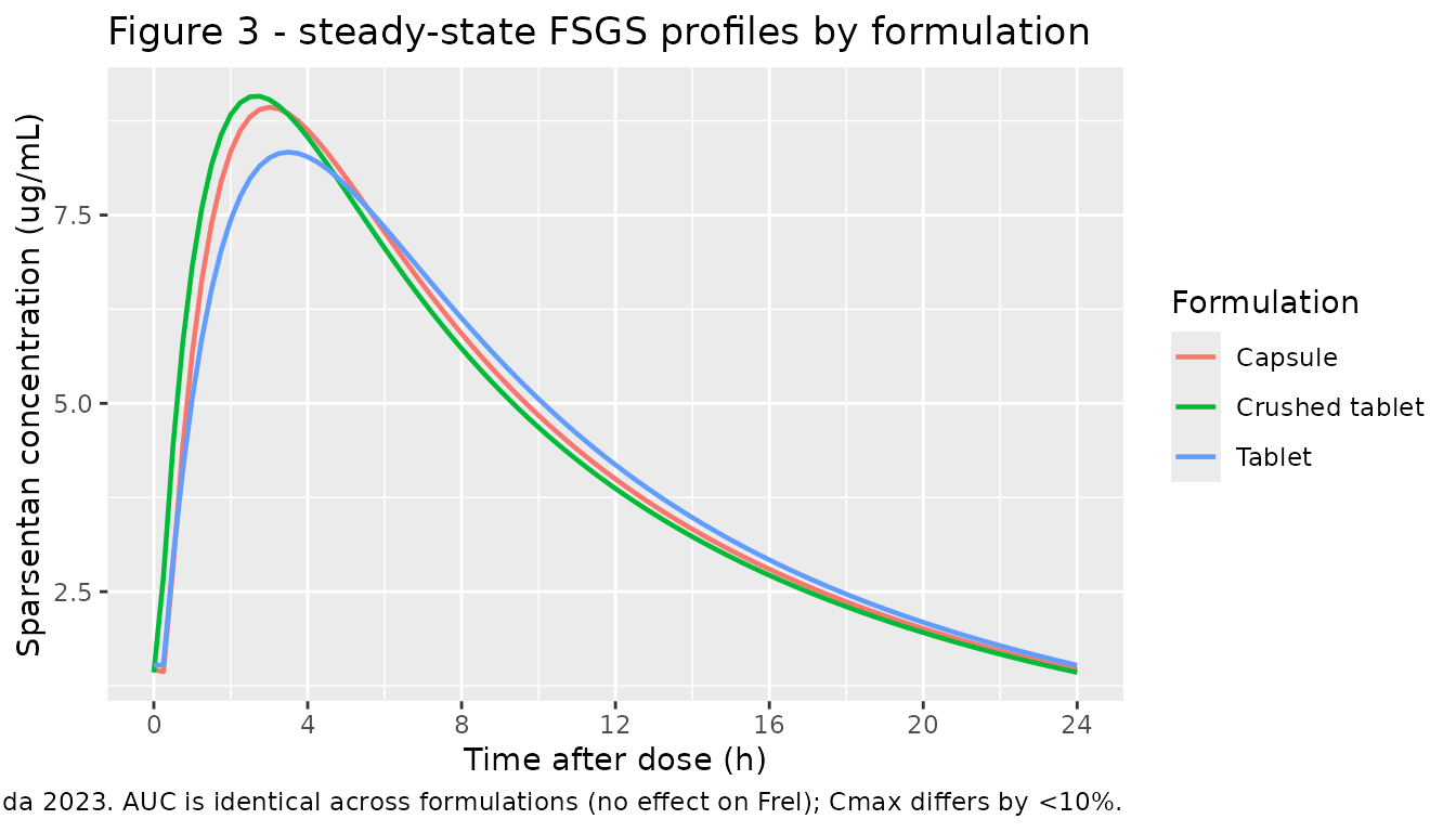

Figure 1 - VPC after a single dose and at steady state

set.seed(20230815)
N_VPC <- 150L   # per arm; well under the 200/arm cap

# Healthy-volunteer arm: single 400 mg tablet, dense sampling to 72 h.
# Race and sex are drawn to match the healthy-subject column of Table 1
# (26.3% female; 59.7% White / 37.7% Black / 1.7% Asian).
hv_ids <- tibble::tibble(
  id         = seq_len(N_VPC),
  SEXF       = rbinom(N_VPC, 1, 0.263),
  race       = sample(c("White", "Black", "Asian"), N_VPC, replace = TRUE,
                      prob = c(0.597, 0.377, 0.017)),
  ALP        = pmax(30, rlnorm(N_VPC, log(65), 0.28)),
  CRCL       = pmax(70, rlnorm(N_VPC, log(123), 0.21))
) |>
  dplyr::mutate(RACE_BLACK = as.integer(race == "Black"),
                RACE_ASIAN = as.integer(race == "Asian")) |>
  dplyr::select(-race)

# FSGS arm: 800 mg once daily to steady state; observed over the last
# dosing interval. Table 1 FSGS column: 44.3% female; 75.3% White /
# 7.7% Black / 11.3% Asian; median ALKP 73 U/L, median CrCL 78 mL/min.
fsgs_ids <- tibble::tibble(
  id         = 1000L + seq_len(N_VPC),
  SEXF       = rbinom(N_VPC, 1, 0.443),
  race       = sample(c("White", "Black", "Asian"), N_VPC, replace = TRUE,
                      prob = c(0.753, 0.077, 0.113)),
  ALP        = pmax(25, rlnorm(N_VPC, log(73), 0.42)),
  CRCL       = pmax(26, rlnorm(N_VPC, log(78), 0.45))
) |>
  dplyr::mutate(RACE_BLACK = as.integer(race == "Black"),
                RACE_ASIAN = as.integer(race == "Asian")) |>
  dplyr::select(-race)

vpc_events <- dplyr::bind_rows(
  make_arm("Healthy volunteers, single 400 mg tablet", N_VPC, 400,
           obs_times = c(seq(0, 12, by = 0.5), seq(14, 72, by = 2)),
           dose_times = 0, id_offset = 0L,
           covariates = list(FORM_TABLET = 1), per_id = hv_ids),
  make_arm("FSGS patients, 800 mg tablet QD steady state", N_VPC, 800,
           obs_times = seq(13 * 24, 14 * 24, by = 0.5),
           dose_times = seq(0, 13 * 24, by = 24), id_offset = 1000L,
           covariates = list(FORM_TABLET = 1), per_id = fsgs_ids)
)
stopifnot(!anyDuplicated(unique(vpc_events[, c("id", "time", "evid")])))

sim_vpc <- rxode2::rxSolve(
  mod, events = vpc_events,
  keep = c("arm", "CRCL", "ALP", "SEXF", "RACE_BLACK", "RACE_ASIAN")
) |>
  as.data.frame() |>
  dplyr::mutate(
    tad = ifelse(grepl("^FSGS", arm), time - 13 * 24, time)
  )

# Guard: the per-subject covariates must actually reach the solver. If the
# `per_id` join or the `keep =` plumbing silently dropped them, every subject
# would share the default covariate values and the VPC would be quietly wrong
# with no visible symptom.
stopifnot(
  dplyr::n_distinct(sim_vpc$CRCL)       > 1,
  dplyr::n_distinct(sim_vpc$ALP)        > 1,
  dplyr::n_distinct(sim_vpc$SEXF)       == 2,
  dplyr::n_distinct(sim_vpc$RACE_BLACK) == 2
)

sim_vpc |>
  dplyr::filter(tad > 0) |>
  dplyr::group_by(arm, tad) |>
  dplyr::summarise(
    Q05 = quantile(Cc, 0.05, na.rm = TRUE),
    Q50 = quantile(Cc, 0.50, na.rm = TRUE),
    Q95 = quantile(Cc, 0.95, na.rm = TRUE),
    .groups = "drop"
  ) |>
  ggplot(aes(tad, Q50)) +
  geom_ribbon(aes(ymin = Q05, ymax = Q95), alpha = 0.25, fill = "steelblue") +
  geom_line(linewidth = 0.7) +
  facet_wrap(~arm, scales = "free_x") +
  scale_y_log10() +
  labs(x = "Time after dose (h)",
       y = "Sparsentan concentration (ug/mL)",
       title = "Figure 1 - simulated concentration percentiles",
       caption = paste(
         "Mirrors the layout of Figure 1 of Wada 2023 (panels a and d).",
         "Ribbon is the 5th-95th percentile of the model prediction;",
         "line is the median. Observed data are not publicly available."))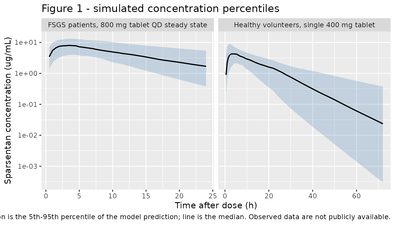

PKNCA validation

# Steady-state arm plus a post-steady-state washout, so that (a) AUC0-tau,
# Cmax and Cmin come from a genuine steady-state dosing interval, and (b) the
# terminal half-life is estimated after the auto-induction is complete
# (the published 9.6 h is explicitly the steady-state value).
LAST_DOSE <- 13 * 24
TAU       <- 24

nca_settings <- list(
  # Reference subject of Table 2 footnote b, at 400 mg: gives the published
  # steady-state terminal half-life of 9.6 h.
  list(lbl = "Reference subject, 400 mg QD", dose = 400, cov = list()),
  # The combined high-exposure FSGS covariate case of the Discussion:
  # White female, CrCL 41 mL/min (5th pct), ALKP 141 U/L (95th pct),
  # concomitant moderate CYP3A4 inhibitor, 800 mg/day.
  list(lbl = "High-exposure FSGS, 800 mg QD", dose = 800,
       cov = list(SEXF = 1, CRCL = 41, ALP = 141, FORM_TABLET = 1,
                  CONMED_CYP3A4_INH_MOD = 1))
)

nca_events <- dplyr::bind_rows(lapply(seq_along(nca_settings), function(i) {
  s <- nca_settings[[i]]
  make_arm(s$lbl, 1, s$dose,
           obs_times = c(seq(LAST_DOSE, LAST_DOSE + TAU, by = 0.25),
                         seq(LAST_DOSE + TAU + 2, LAST_DOSE + TAU + 96, by = 2)),
           dose_times = seq(0, LAST_DOSE, by = 24),
           id_offset = (i - 1L) * 10L,
           covariates = s$cov)
}))

sim_nca_raw <- rxode2::rxSolve(mod, events = nca_events, omega = NA,
                               keep = "arm") |>
  as.data.frame()
#> Warning: multi-subject simulation without without 'omega'

sim_nca <- sim_nca_raw |>
  dplyr::filter(!is.na(Cc)) |>
  dplyr::select(id, time, Cc, arm)

# Defensive time-zero record (extravascular: pre-dose Cc = 0), so PKNCA never
# emits "Requesting an AUC range starting (0) before the first measurement".
sim_nca <- dplyr::bind_rows(
  sim_nca,
  sim_nca |> dplyr::distinct(id, arm) |>
    dplyr::mutate(time = 0, Cc = 0)
) |>
  dplyr::distinct(id, arm, time, .keep_all = TRUE) |>
  dplyr::arrange(id, arm, time)

dose_df <- nca_events |>
  dplyr::filter(evid == 1) |>
  dplyr::select(id, time, amt, arm)

conc_obj <- PKNCA::PKNCAconc(sim_nca, Cc ~ time | arm + id,
                             concu = "ug/mL", timeu = "h")
dose_obj <- PKNCA::PKNCAdose(dose_df, amt ~ time | arm + id, doseu = "mg")

intervals <- data.frame(
  start     = c(LAST_DOSE, LAST_DOSE),
  end       = c(LAST_DOSE + TAU, LAST_DOSE + TAU + 96),
  cmax      = c(TRUE,  FALSE),
  tmax      = c(TRUE,  FALSE),
  cmin      = c(TRUE,  FALSE),
  auclast   = c(TRUE,  FALSE),
  half.life = c(FALSE, TRUE)
)

nca_res <- PKNCA::pk.nca(PKNCA::PKNCAdata(conc_obj, dose_obj,
                                          intervals = intervals))

Comparison against published NCA

PKNCA emits dependency rows into whichever interval needs them, so the result frame is filtered on start / end as well as on PPTESTCD before the comparison - otherwise a parameter computed in both intervals would be averaged across them.

res_tbl <- as.data.frame(nca_res$result)

sim_long <- dplyr::bind_rows(
  res_tbl |>
    dplyr::filter(start == LAST_DOSE, end == LAST_DOSE + TAU,
                  PPTESTCD %in% c("cmax", "tmax", "cmin", "auclast")),
  res_tbl |>
    dplyr::filter(start == LAST_DOSE, end == LAST_DOSE + TAU + 96,
                  PPTESTCD == "half.life")
) |>
  dplyr::select(arm, PPTESTCD, PPORRES)

# Only two NCA-scale quantities are published numerically: the steady-state
# terminal half-life (Table 2) and the steady-state AUC of the combined
# high-exposure covariate case (Discussion). Supplying the reference in long
# form lets the unreported combinations be omitted rather than padded with NA.
published_nca <- tibble::tribble(
  ~arm,                            ~PPTESTCD,   ~PPORRES,
  "Reference subject, 400 mg QD",  "half.life",      9.6,
  "High-exposure FSGS, 800 mg QD", "auclast",      193.0
)

cmp <- nlmixr2lib::ncaComparisonTable(
  simulated     = sim_long,
  reference     = published_nca,
  by            = "arm",
  units         = c(half.life = "h", auclast = "ug*h/mL"),
  tolerance_pct = 20
)

knitr::kable(
  cmp,
  caption = "Simulated vs. published NCA. * differs from reference by >20%.",
  align   = c("l", "l", "r", "r", "r")
)

Simulated vs. published NCA. * differs from reference by >20%.

NCA parameter	arm	Reference	Simulated	% diff
AUClast (ug*h/mL)	High-exposure FSGS, 800 mg QD	193	212	+10.0%
t½ (h)	Reference subject, 400 mg QD	9.6	9.48	-1.2%

attr(cmp, "footnote")
#> NULL

The remaining steady-state NCA quantities are reported by Wada 2023 only graphically (Figure 2 tornado plots, Figures S2-S3 boxplots), so they are shown below for reference rather than compared numerically.

res_tbl |>
  dplyr::filter(start == LAST_DOSE, end == LAST_DOSE + TAU,
                PPTESTCD %in% c("cmax", "cmin", "tmax", "auclast")) |>
  dplyr::mutate(PPTESTCD = nlmixr2lib::ncaParamLabel(PPTESTCD)) |>
  dplyr::select(arm, PPTESTCD, PPORRES) |>
  tidyr::pivot_wider(names_from = PPTESTCD, values_from = PPORRES) |>
  dplyr::rename("Arm" = arm) |>
  knitr::kable(
    digits  = 3,
    caption = paste(
      "Simulated steady-state NCA over the final 24 h dosing interval",
      "(typical-value subjects, no between-subject variability).")
  )

Simulated steady-state NCA over the final 24 h dosing interval (typical-value subjects, no between-subject variability).

Arm	AUClast	Cmax	Cmin	Tmax
High-exposure FSGS, 800 mg QD	212.287	12.605	5.273	4
Reference subject, 400 mg QD	78.281	6.424	1.114	3

Assumptions and deviations

• The Day variable in the auto-induction term is taken to be the whole-day index since the first dose, 0 on the first dosing day. Wada 2023 writes the time-dependent clearance as CL(t) = CL0 + dCL * (1 - exp(-k_induction * Day)) (Methods; Table S3) but does not define Day. This model derives it as floor(time / 24), which assumes time = 0 is the first dose. Three lines of evidence support the whole-day-index reading over a continuous days-since-first-dose reading:
  1. the induction half-life is fixed at 0.001 day, so under a continuous reading the term would reach 1 within ~2 minutes of the first dose and the pre-induction CL0 = 3.88 L/h would not be estimable at all - yet the paper reports it with 4.6% RSE and dCL with 13.6% RSE; (2) the paper reports 3.88 L/h and 5.12 L/h as two separately realised values (“CL/F was 3.88 L/h after a single 400-mg dose, increasing to 5.12 L/h at steady-state”), which only a step at a day boundary produces; and (3) the prose describes “a rapid increase to steady-state occurring after the first dose during multiple-dose regimens” (Results, base model) and an effect “occurring instantly after the first dose” (Discussion). If a downstream user’s event table does not start at the first dose, Day must be supplied differently.
• The additive residual SD is expressed in the model’s concentration scale. The model integrates amounts in mg with volumes in L, so Cc is in mg/L = ug/mL. Wada 2023 fixes the additive residual SD at 2 ng/mL (the assay LLOQ), entered here as addSd = 0.002 ug/mL. No scaling constant appears in model(); the paper itself reports exposures in ug/mL*h.
• Residual-error terms are read as standard deviations, not variances. Table 2 labels both rows explicitly as SDs (“SD of proportional error”, “SD of additive error (ng/mL)”), and the additive value equals the LLOQ, which is only meaningful as an SD.
• The reported “IIV (%)” column is sqrt(omega^2), not a log-normal CV. sqrt(0.156) = 39.5%, sqrt(0.234) = 48.4%, sqrt(0.474) = 68.9% reproduce Table 2’s IIV column exactly, so the “Variance” rows are used verbatim with no omega^2 = log(1 + CV^2) conversion.
• The between-subject random effect on clearance multiplies the whole typical-value expression (auto-induction bracket times covariate effects), matching the paper’s theta_i = theta_typical * exp(eta_i) statement and the layout of Table S3. This costs full mu-referencing on cl (the composite is additive in CL, so exp(lcl + etalcl) alone cannot express it), which matters only if the model is re-estimated.
• No IIV on Q/F, Vp/F, or Tlag, and no eta correlations. Table 2 reports “-” or “NA” in the IIV column for those parameters and reports no covariance block, so OMEGA is diagonal.
• The CYP3A4-inhibitor covariate is retained even though it is absent from the paper’s list of six backward-elimination survivors. Results “Final model” names ALKP, CrCL and sex on CL, race on Vc, and formulation on Tlag and Ka as the six retained covariate-parameter relationships, but the Abstract, Table 2, Table 3, Table S3, Figure 2 and the Discussion all carry the moderate and strong CYP3A4 inhibitor effects on CL - the latter being the paper’s headline finding. The inhibitor effects were evidently included a priori rather than via the stepwise search. Table 2 and Table S3 are treated as authoritative.
• Weak CYP3A4 inhibitors fall in the reference category. 12.8% of the cohort received a weak inhibitor; no coefficient is published for that stratum, so those subjects are pooled with the no-inhibitor reference.
• Subjects of “Multiple” (0.7%) or “Other” (2.2%) race fall in the White reference category for the Vc effect, because Wada 2023 publishes coefficients only for Black or African American and Asian.
• The Frel branch boundary differs between two places in the source. Table 2’s note reads “if dose >= 200 mg” / “if dose < 200 mg” while Table S3 reads “if Dose > 200 mg” / “if Dose <= 200 mg”. The two readings agree numerically because both branches give the same value at exactly 200 mg. The model uses max(DOSE, 200), which reproduces both.
• CrCL is raw (absolute) Cockcroft-Gault mL/min, not BSA-normalised, unlike the CRCL register default of mL/min/1.73 m^2. The paper states Cockcroft-Gault explicitly and the reference value 112 mL/min matches the Table 1 overall median in mL/min.
• Virtual-cohort covariate distributions are assumptions. Wada 2023 publishes only medians, means, SDs and ranges (Table 1), not joint distributions, so the VPC arms draw ALP and CRCL from independent log-normals matched to the published medians and coefficients of variation, and sex and race from independent Bernoulli / categorical draws matched to the published percentages. Correlations among covariates (notably between CrCL, sex and age) are not reproduced.
• **The 193 ug/mL*h combined-covariate AUC is reproduced within ~10%, but the paper’s accompanying “82% increase” is internally inconsistent with its own parameters.** The Discussion states that for a White female FSGS patient with CrCL at the 5th percentile (41 mL/min), ALKP at the 95th percentile (141 U/L), and concomitant moderate CYP3A4 inhibition, the steady-state AUC after 800 mg/day would be 193 ug/mLh, “representing an 82% increase in exposure”. Applying the Table S3 equations to the typical FSGS subject gives a baseline steady-state AUC of 106 ug/mLh, and 193 / 106 = 1.82 - so the paper’s ratio and its baseline are mutually consistent. However, the same equations applied to the covariate combination itself give ~212 ug/mLh (a 100% increase), because the product of the four covariate factors is 0.501 rather than the 0.549 implied by 193 ug/mLh. The discrepancy is confined to this illustrative Discussion sentence; every value in Tables 2, 3 and S3 is reproduced exactly (see the tables above). No parameter was tuned to close the gap.
• No published numeric NCA table exists for the main dose groups. Wada 2023 reports steady-state Cmax, Cmin and AUC only graphically (Figure 2 tornado plots; Figures S2-S3 boxplots) and as percent changes (Results “Impact of covariates on sparsentan exposure”). The NCA comparison above is therefore limited to the two numerically published quantities: the steady-state terminal half-life and the combined-covariate steady-state AUC.
• Inter-occasion variability is not modelled. The paper does not report an IOV component; several studies had crossover periods (Table 1 footnote a) but no occasion random effect is published.
• Hepatic impairment is not a covariate. Wada 2023 tested ALKP, ALT, AST and total bilirubin in place of a hepatic-function classification and retained only ALKP, so the 16 hepatic-impairment subjects are described by the same structural model with their own laboratory values.