Iadademstat (ORY-1001) in vitro to in vivo QSP model (Bouhaddou 2020)

Model and source

Bouhaddou 2020 builds a semimechanistic PK/PD model of iadademstat (ORY-1001), a covalent inhibitor of the histone demethylase LSD1 (KDM1A), in the NCI-H510A small-cell lung cancer (SCLC) cell line. The model is trained almost entirely on cell-culture data and then used to predict xenograft tumour growth in mice. The authors built two models, and the paper contributes two files to nlmixr2lib:

mod_vitro <- rxode2::rxode(readModelDb("Bouhaddou_2020_iadademstat_invitro"))
mod_vivo <- rxode2::rxode(readModelDb("Bouhaddou_2020_iadademstat_mouse"))

The two model files contributed by Bouhaddou 2020.

nlmixr2lib model	Role
Bouhaddou_2020_iadademstat_invitro	In vitro PD model: constant drug concentration -> LSD1 target engagement -> GRP mRNA -> proliferating / quiescent cell switch (Figures 2-3)
Bouhaddou_2020_iadademstat_mouse	In vivo PK/PD model: oral two-compartment PK with dose-dependent bioavailability, unbound plasma concentration driving the same PD model; only kP re-estimated (Figures 4-5)

• Citation: Bouhaddou M, Yu LJ, Lunardi S, Stamatelos SK, Mack F, Gallo JM, Birtwistle MR, Walz AC. (2020). Predicting In Vivo Efficacy from In Vitro Data: Quantitative Systems Pharmacology Modeling for an Epigenetic Modifier Drug in Cancer. Clin Transl Sci 13(2):419-429. doi:10.1111/cts.12727. Parameter values from Supplementary Table S2 and the deposited MATLAB code (Supplementary zip, vivo_model/rateconstants_vivo_BEST.txt, RunModelVivo.m).
• Article: https://doi.org/10.1111/cts.12727
• PubMed Central: https://www.ncbi.nlm.nih.gov/pmc/articles/PMC7070804/

The paper’s display equations (Eqs. 1-20) give the structure; the parameter values are in Supplementary Tables S1 (initial conditions) and S2 (parameters). The authors also deposited their MATLAB code, the fitted parameter files and the experimental data as a supplementary zip (code_Bouhaddouetal_pub). The deposit settles one printed-equation defect (Eq. 1, see Assumptions and deviations) and supplies the observed data that the figure replications below are compared against.

Population

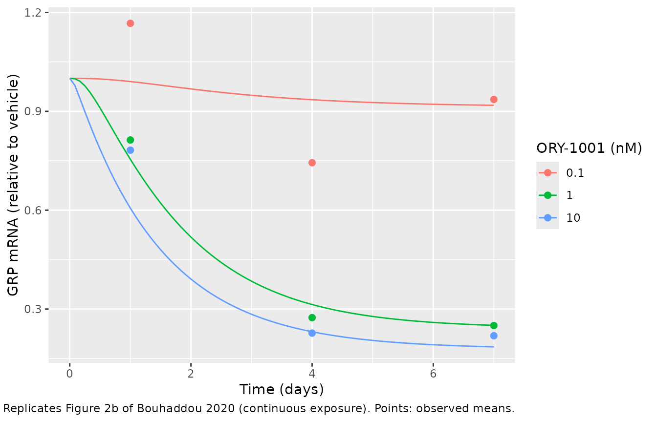
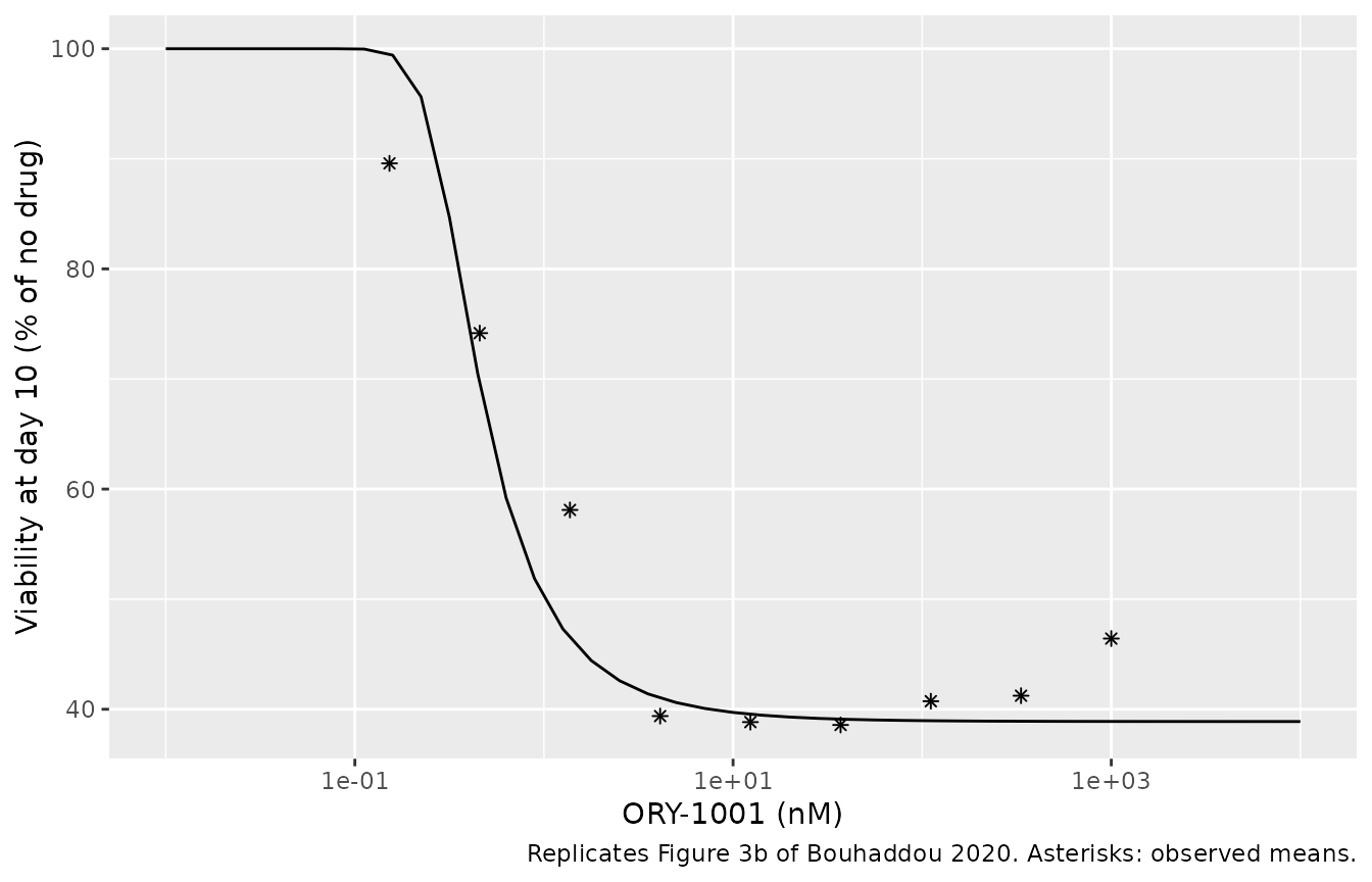
• In vitro: NCI-H510A cells. Target engagement was measured by an ELISA-based free/total LSD1 chemoprobe assay after 24 h exposure to 0.6, 3 or 15 nM followed by 3 days of wash-out; GRP mRNA by TaqMan RT-qPCR after continuous 0.1, 1 or 10 nM for up to 7 days and after 5 nM pulsed (3 days on / 7 off) or continuous (10 days) exposure; growth and viability by alamarBlue in 96-well plates seeded at 8000 cells per well, over 10 days. Three biological replicates per condition.
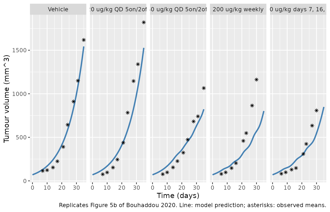
• In vivo: female athymic nude mice, 7-8 weeks old, implanted subcutaneously with 5 million NCI-H510A cells. PK was measured in tumour-free mice after single oral doses (3 mice per time point); efficacy in five arms of 13-15 mice (vehicle, 20 and 40 ug/kg once daily 5-on/2-off, 200 ug/kg weekly, 400 ug/kg on days 7, 16 and 23). Mouse plasma fraction unbound was 0.75.

The same information is available programmatically via the population metadata, e.g. readModelDb("Bouhaddou_2020_iadademstat_mouse")()$population.

Source trace

Every ini() value carries an in-file comment naming its source. The table collects them. “Code” refers to the deposited MATLAB files.

Equation / parameter	Value	Source location
Depot, central, peripheral ODEs	n/a	Eqs. 1-3 (p. 420-421); RunModelVivo.m
Dose-dependent bioavailability F = D / (D50 + D)	n/a	Eq. 1 as implemented in RunModelVivo.m (Xup = (X0/(D50+X0))*X0)
Cc = central / V	n/a	Eq. 5
Unbound active concentration roc = Cc * fu * 1000 / MW (nM)	n/a	Eq. 4; RunModelVivo.m (fac_ng2nM)
d/dt(roc) = 0 (in vitro)	n/a	Eq. 6
Bound LSD1 ODE, unbound LSD1, TE	n/a	Eqs. 7-9 (p. 422)
GRP mRNA ODE, kmax = -m*GRP + b, m = b - kdeg	n/a	Eqs. 10-12 (p. 422)
Proliferating / quiescent ODEs and switching rates	n/a	Eqs. 13-20 (p. 422)
lka	log(0.88205) 1/h	Table S2
lcl	log(117.66) mL/h	Table S2 (‘kCL’); code CL = CLml/V
lvc	log(577.49) mL	Table S2
lk12, lk21	log(0.47004), log(0.25469) 1/h	Table S2
ld50	log(1123.9) ng	Table S2
fu	0.75 (measured)	Table S2; Results p. 424
mw	230.4 g/mol	Code rateconstants_vivo_BEST.txt
ki	19 nM (measured)	Table S2
lkinact	log(0.87052) 1/h	Table S2
lvmax_lsd1b, lkm_lsd1b	log(0.03515) nM/h, log(0.9028) nM	Table S2
llsd1tot	log(3.0833) nM	Table S2
lte50, hill_te	log(26.513) %, 2.0819	Table S2
lkdeg_grp, b_grp	log(0.025567) 1/h, 0.083048 1/h	Table S2
lkp	log(0.023) in vitro; log(0.0037) in vivo (1/h)	Table S2
lk50p	log(100000)	Table S2
lkmaxpq, lkmaxqp	log(0.5932), log(4.4908) 1/h	Table S2
k50pq, k50qp	0.8836, 0.99897	Table S2
hill_pq, hill_qp	3.8313, 37.455	Table S2
bs	0.033328	Table S2
prolif0	8000 cells in vitro; 70 mm^3 in vivo	Table S1
grp(0)	1	Table S1

Reproduction gate: an independent implementation of the authors’ code

The deposited RunModelVivo.m is simulated here a second time from a separate transcription of its right-hand side (compiled on its own, not read from the model file), following the MATLAB driver literally: 35 consecutive 24-hour integrations, the depot overwritten with the dose at the start of each dosing day, and the bioavailability correction X0 <- X0 * X0 / (D50 + X0) applied to the depot at the start of every 24-hour chunk (RunDosingRegVivo.m). The nlmixr2lib model instead adds each dose through a single f(depot). The two differ only by the negligible depot residue left after 24 h (exp(-0.882 * 24) ~ 6e-10), so they must agree to solver precision.

# Parameter vector in the order of rateconstants_vivo_BEST.txt.
k_vivo <- c(
  Ki = 19, kinact = 0.87052, vm = 0.03515, km = 0.9028, LSD1_0 = 3.0833,
  k50 = 26.513, n = 2.0819, kd = 0.025567, b = 0.083048, kP = 0.0037,
  k50P = 1e5, kmaxPQ = 0.5932, kmaxQP = 4.4908, k50PQ = 0.8836,
  k50QP = 0.99897, nPQ = 3.8313, nQP = 37.455, bs = 0.033328,
  ka = 0.88205, k12 = 0.47004, k21 = 0.25469, V = 577.49, D50 = 1123.9,
  CLml = 117.66, fu = 0.75, MW = 230.4
)

# Right-hand side of RunModelVivo.m's createODEs(), transcribed separately from
# the model file; the ROc ODE is the authors' own (fac_ng2nM times dQc/dt).
# States are declared in the MATLAB order (ROc, LSD1B, GRP, P, Q, X, Qc, Qp).
matlab_ode <- rxode2::rxode2("
  CL = CLml / V;
  fac = (1000 / MW) / V * fu;
  dQc = ka * X - CL * Qc - k12 * Qc + k21 * Qp;
  d/dt(ROc) = dQc * fac;
  LSD1U = LSD1_0 - LSD1B;
  d/dt(LSD1B) = -LSD1B * (vm / (km + LSD1B)) + kinact * ROc / (Ki + ROc) * LSD1U;
  TE = LSD1B / LSD1_0 * 100;
  m = b - kd;
  kmax = -m * GRP + b;
  d/dt(GRP) = kmax * (k50^n / (k50^n + TE^n)) - kd * GRP;
  vP = kP * (1 - P / (k50P + P)) * P;
  BM = abs(1 - GRP);
  vPQ = kmaxPQ * BM^nPQ / (k50PQ^nPQ + BM^nPQ) * P;
  BMQP = 1 - BM;
  vQP = kmaxQP * (BMQP^nQP / (k50QP^nQP + BMQP^nQP) + bs) * Q;
  d/dt(P) = vP - vPQ + vQP;
  d/dt(Q) = vPQ - vQP;
  d/dt(X) = -ka * X;
  d/dt(Qc) = dQc;
  d/dt(Qp) = k12 * Qc - k21 * Qp;
")

# RunDosingRegVivo.m: day-by-day driver; dose_ugkg converted with a 0.025 kg mouse.
matlab_regimen <- function(dose_ugkg, dose_days, k, total_days = 35) {
  y <- c(ROc = 0, LSD1B = 0, GRP = 1, P = 70, Q = 0, X = 0, Qc = 0, Qp = 0)
  pars <- k[setdiff(names(k), "D50")]
  day_grid <- rxode2::et(seq(0, 24, by = 1))
  out <- list()
  for (i in seq_len(total_days)) {
    if (i %in% dose_days) y[["X"]] <- dose_ugkg * 1e3 * 0.025
    y[["X"]] <- y[["X"]] / (k[["D50"]] + y[["X"]]) * y[["X"]]
    s <- as.data.frame(rxode2::rxSolve(matlab_ode, params = pars, events = day_grid,
                                       inits = y, rtol = 1e-10, atol = 1e-12))
    keep <- seq_len(nrow(s) - 1L)
    out[[i]] <- data.frame(
      time = s$time[keep] + (i - 1) * 24,
      Cc = s$Qc[keep] / k[["V"]],
      TE = s$LSD1B[keep] / k[["LSD1_0"]] * 100,
      grp = s$GRP[keep],
      tumor_vol = s$P[keep] + s$Q[keep]
    )
    y <- unlist(s[nrow(s), names(y)])
  }
  dplyr::bind_rows(out)
}

# MATLAB day indices of dosing (RunDosingRegVivo.m, `dayson`).
regimens <- tibble::tibble(
  arm = c(
    "Vehicle", "20 ug/kg QD 5on/2off", "40 ug/kg QD 5on/2off",
    "200 ug/kg weekly", "400 ug/kg days 7, 16, 23"
  ),
  dose_ugkg = c(0, 20, 40, 200, 400),
  dose_days = list(
    integer(), c(14:18, 21:25, 28:32, 35), c(14:18, 21:25, 28:32, 35),
    c(7, 14, 21, 28), c(7, 16, 23)
  )
) |>
  dplyr::mutate(arm = factor(arm, levels = arm))

# nlmixr2lib event table: dose on MATLAB day index i is given at (i - 1) * 24 h.
# Observations are on ODE states (prolif), so every algebraic output is returned.
regimen_events <- function(dose_ugkg, dose_days, arm_id) {
  obs <- data.frame(id = arm_id, time = seq(0, 35 * 24, by = 1), evid = 0, amt = 0, cmt = "prolif")
  if (length(dose_days) == 0L || dose_ugkg == 0) {
    return(obs)
  }
  dose <- data.frame(
    id = arm_id, time = (dose_days - 1) * 24, evid = 1,
    amt = dose_ugkg * 1e3 * 0.025, cmt = "depot"
  )
  dplyr::bind_rows(dose, obs) |> dplyr::arrange(time, dplyr::desc(evid))
}

ev_vivo <- dplyr::bind_rows(lapply(seq_len(nrow(regimens)), function(i) {
  regimen_events(regimens$dose_ugkg[i], regimens$dose_days[[i]], i)
}))
sim_vivo <- rxode2::rxSolve(mod_vivo, ev_vivo, rtol = 1e-10, atol = 1e-12) |>
  as.data.frame() |>
  dplyr::mutate(arm = regimens$arm[id])

ref_vivo <- dplyr::bind_rows(lapply(seq_len(nrow(regimens)), function(i) {
  matlab_regimen(regimens$dose_ugkg[i], regimens$dose_days[[i]], k_vivo) |>
    dplyr::mutate(arm = regimens$arm[i])
}))

cmp_vivo <- dplyr::inner_join(sim_vivo, ref_vivo, by = c("arm", "time"), suffix = c("", "_ref"))
stopifnot(nrow(cmp_vivo) == 5 * 35 * 24)
repro <- cmp_vivo |>
  dplyr::group_by(arm) |>
  dplyr::summarise(
    tumor_vol = max(abs(tumor_vol / tumor_vol_ref - 1)),
    grp = max(abs(grp - grp_ref)),
    TE = max(abs(TE - TE_ref)),
    Cc = max(abs(Cc - Cc_ref)) / max(max(Cc_ref), 1e-12),
    .groups = "drop"
  )
knitr::kable(
  repro |>
    dplyr::rename(
      "Arm" = arm, "tumor_vol (max rel. diff)" = tumor_vol,
      "GRP (max abs. diff)" = grp, "TE (max abs. diff, %)" = TE,
      "Cc (max diff / Cmax)" = Cc
    ),
  digits = 8,
  caption = "nlmixr2lib model vs a separate transcription of the authors' MATLAB driver."
)

nlmixr2lib model vs a separate transcription of the authors’ MATLAB driver.

Arm	tumor_vol (max rel. diff)	GRP (max abs. diff)	TE (max abs. diff, %)	Cc (max diff / Cmax)
Vehicle	0	0	0e+00	0
20 ug/kg QD 5on/2off	0	0	2e-08	0
40 ug/kg QD 5on/2off	0	0	3e-08	0
200 ug/kg weekly	0	0	3e-08	0
400 ug/kg days 7, 16, 23	0	0	3e-08	0

# Both sides solve the same deterministic ODE with the same parameters, so the
# difference is numerical error only and a tight bound is correct (a
# mis-transcribed parameter or a wrong dose conversion moves these by >1%).
stopifnot(
  max(repro$tumor_vol) < 1e-4,
  max(repro$grp) < 1e-4,
  max(repro$TE) < 1e-3,
  max(repro$Cc) < 1e-4
)

In vitro model: Figures 2 and 3

In the cell-culture experiments the drug concentration is constant while it is on (Eq. 6). Exposure starts with a dose of the concentration (nM) into roc and ends with a replacement event (evid = 5, amt = 0), which is how RunModelVitro.m models the wash-off (y2(1) = 0).

# One well: exposure to conc_nM from time 0 to t_off (h), observed on `obs_times`.
vitro_events <- function(conc_nM, t_off, obs_times, well) {
  ev <- data.frame(id = well, time = obs_times, evid = 0, amt = 0, cmt = "prolif")
  if (conc_nM > 0) {
    ev <- dplyr::bind_rows(
      data.frame(id = well, time = 0, evid = 1, amt = conc_nM, cmt = "roc"),
      ev
    )
    if (is.finite(t_off)) {
      ev <- dplyr::bind_rows(
        ev,
        data.frame(id = well, time = t_off, evid = 5, amt = 0, cmt = "roc")
      )
    }
  }
  dplyr::arrange(ev, time, dplyr::desc(evid == 0))
}

Figure 2a – target engagement after a 24-hour pulse

te_obs <- tibble::tribble(
  ~conc, ~time, ~TE,
  0.6, 24, 58.24, 0.6, 48, 11.81, 0.6, 72, 12.97, 0.6, 96, 10.20,
  3, 24, 81.07, 3, 48, 65.96, 3, 72, 47.79, 3, 96, 34.19,
  15, 24, 84.76, 15, 48, 68.99, 15, 72, 65.23, 15, 96, 50.91
)
concs_te <- c(0.6, 3, 15)
ev_te <- dplyr::bind_rows(lapply(seq_along(concs_te), function(i) {
  vitro_events(concs_te[i], 24, seq(0, 96, by = 1), i)
}))
sim_te <- rxode2::rxSolve(mod_vitro, ev_te) |>
  as.data.frame() |>
  dplyr::mutate(conc = concs_te[id])

ggplot(sim_te, aes(time / 24, TE, colour = factor(conc))) +
  geom_line() +
  geom_point(data = te_obs, size = 2) +
  labs(
    x = "Time (days)", y = "Target engagement (%)", colour = "ORY-1001 (nM)",
    caption = "Replicates Figure 2a of Bouhaddou 2020 (24 h exposure, then wash-off). Points: observed means."
  )

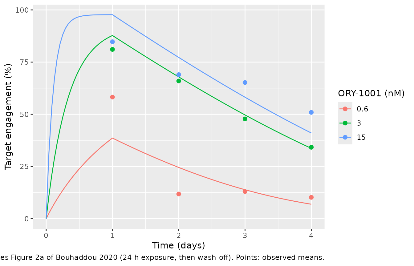
Figure 2b and 2c – GRP mRNA under continuous and pulsed exposure

grp_obs <- tibble::tribble(
  ~conc, ~time, ~grp,
  0.1, 24, 1.167, 0.1, 96, 0.744, 0.1, 168, 0.936,
  1, 24, 0.813, 1, 96, 0.274, 1, 168, 0.250,
  10, 24, 0.782, 10, 96, 0.227, 10, 168, 0.219
)
concs_grp <- c(0.1, 1, 10)
ev_grp <- dplyr::bind_rows(lapply(seq_along(concs_grp), function(i) {
  vitro_events(concs_grp[i], Inf, seq(0, 168, by = 2), i)
}))
sim_grp <- rxode2::rxSolve(mod_vitro, ev_grp) |>
  as.data.frame() |>
  dplyr::mutate(conc = concs_grp[id])

ggplot(sim_grp, aes(time / 24, grp, colour = factor(conc))) +
  geom_line() +
  geom_point(data = grp_obs, size = 2) +
  labs(
    x = "Time (days)", y = "GRP mRNA (relative to vehicle)", colour = "ORY-1001 (nM)",
    caption = "Replicates Figure 2b of Bouhaddou 2020 (continuous exposure). Points: observed means."
  )

# Figure 2c: 5 nM for 3 days then 7 days off, versus 10 days continuous.
ev_wo <- dplyr::bind_rows(
  vitro_events(5, 72, seq(0, 240, by = 2), 1),
  vitro_events(5, Inf, seq(0, 240, by = 2), 2)
)
sim_wo <- rxode2::rxSolve(mod_vitro, ev_wo) |>
  as.data.frame() |>
  dplyr::mutate(schedule = c("3 days on, 7 off", "10 days on")[id])
wo_day10 <- sim_wo |>
  dplyr::filter(time == 240) |>
  dplyr::select(schedule, grp) |>
  dplyr::mutate(observed = c(1.10, 0.19)[match(schedule, c("3 days on, 7 off", "10 days on"))])
knitr::kable(
  wo_day10 |> dplyr::rename("Schedule" = schedule, "Simulated GRP, day 10" = grp, "Observed GRP, day 10" = observed),
  digits = 3,
  caption = "Figure 2c bar plot: GRP mRNA at day 10 after 5 nM pulsed or continuous exposure."
)

Figure 2c bar plot: GRP mRNA at day 10 after 5 nM pulsed or continuous exposure.

Schedule	Simulated GRP, day 10	Observed GRP, day 10
3 days on, 7 off	0.986	1.10
10 days on	0.186	0.19

# Structural: a 3-day pulse recovers GRP to baseline by day 10, continuous
# exposure keeps it suppressed (Results p. 423).
stopifnot(
  wo_day10$grp[wo_day10$schedule == "3 days on, 7 off"] > 0.9,
  wo_day10$grp[wo_day10$schedule == "10 days on"] < 0.3
)

Figure 3 – cell growth and viability

# Figure 3a: drug-free growth from 8000 seeded cells.
growth_obs <- tibble::tibble(
  time = c(0, 24, 48, 96, 168, 240),
  cells = c(8501, 24708, 32240, 48168, 130760, 231063)
)
sim_growth <- rxode2::rxSolve(mod_vitro, vitro_events(0, Inf, growth_obs$time, 1)) |>
  as.data.frame()
growth_cmp <- dplyr::mutate(growth_obs, simulated = sim_growth$cell_count)
knitr::kable(
  growth_cmp |> dplyr::rename("Time (h)" = time, "Observed cells" = cells, "Simulated cells" = simulated),
  digits = 0, caption = "Figure 3a: drug-free NCI-H510A growth (observed means from the deposited data)."
)

Figure 3a: drug-free NCI-H510A growth (observed means from the deposited data).

Time (h)	Observed cells	Simulated cells
0	8501	8000
24	24708	13191
48	32240	21155
96	48168	48529
168	130760	121968
240	231063	225924

# Figure 3b: day-10 viability versus concentration, relative to no drug.
cv_obs <- tibble::tibble(
  conc = c(1000, 333.33, 111.11, 37.04, 12.35, 4.115, 1.372, 0.4572, 0.1524),
  viability = 100 * c(109460, 97219, 96041, 90953, 91565, 92858, 137010, 174883, 211239) / 235795
)
conc_grid <- 10^seq(-2, 4, length.out = 41)
ev_cv <- dplyr::bind_rows(lapply(seq_along(conc_grid), function(i) {
  vitro_events(conc_grid[i], Inf, 240, i)
}))
ctrl_10d <- growth_cmp$simulated[growth_cmp$time == 240]
sim_cv <- rxode2::rxSolve(mod_vitro, ev_cv) |>
  as.data.frame() |>
  dplyr::mutate(conc = conc_grid[id], viability = 100 * cell_count / ctrl_10d)

ggplot(sim_cv, aes(conc, viability)) +
  geom_line() +
  geom_point(data = cv_obs, shape = 8) +
  scale_x_log10() +
  labs(
    x = "ORY-1001 (nM)", y = "Viability at day 10 (% of no drug)",
    caption = "Replicates Figure 3b of Bouhaddou 2020. Asterisks: observed means."
  )

# Figure 3c: 5 nM for 3, 5 or 7 days, then off until day 10.
don <- c(3, 5, 7)
ev_pulse <- dplyr::bind_rows(lapply(seq_along(don), function(i) {
  vitro_events(5, 24 * don[i], 240, i)
}))
sim_pulse <- rxode2::rxSolve(mod_vitro, ev_pulse) |>
  as.data.frame() |>
  dplyr::transmute(
    schedule = paste(don[id], "days on"),
    simulated = 100 * cell_count / ctrl_10d,
    # Blue 'Sim' bars of Figure 3c, digitised by the maintainers (+/- 2%).
    published_sim = c(66, 52, 43)[id],
    observed = c(48.9, 35.3, 26.5)[id]
  )
knitr::kable(
  sim_pulse |>
    dplyr::rename(
      "Schedule (5 nM)" = schedule, "Simulated viability (%)" = simulated,
      "Published simulation, Fig. 3c (%)" = published_sim,
      "Observed viability (%)" = observed
    ),
  digits = 1, caption = "Figure 3c: day-10 viability after pulsed 5 nM exposure."
)

Figure 3c: day-10 viability after pulsed 5 nM exposure.

Schedule (5 nM)	Simulated viability (%)	Published simulation, Fig. 3c (%)	Observed viability (%)
3 days on	65.3	66	48.9
5 days on	51.6	52	35.3
7 days on	42.6	43	26.5

The model over-predicts pulsed-exposure viability by about 16 percentage points relative to the observations, and the published simulation bars of Figure 3c show the same gap, so this is a property of the authors’ fit, not of the transcription.

stopifnot(
  # Pulsed viability reproduces the authors' own simulated bars.
  all(abs(sim_pulse$simulated - sim_pulse$published_sim) < 4),
  # Drug-free growth: within 20% of the observed day-10 cell count.
  abs(ctrl_10d / 231063 - 1) < 0.2,
  # Cytostatic plateau: viability saturates near 40-50% at high concentration.
  abs(sim_cv$viability[which.max(sim_cv$conc)] - 46) < 15
)

In vivo model: Figures 4 and 5

Figure 4 – single-dose oral PK in mice

The deposited PK sheet labels its dose column 1, 2 and 500; Plot_PK.m simulates those samples as 20, 40 and 10000 ug/kg, i.e. the column is a multiple of 20 ug/kg. The dose is entered in ng (dose_ugkg * 1000 * 0.025).

pk_obs <- tibble::tribble(
  ~dose_ugkg, ~time, ~Cc,
  20, 1, 0.164, 20, 1, 0.136, 20, 1, 0.0988, 20, 6, 0.043, 20, 6, 0.0217,
  20, 24, 0.0135, 20, 24, 0.0102,
  40, 1, 0.347, 40, 1, 0.392, 40, 1, 0.382, 40, 6, 0.158, 40, 6, 0.201,
  40, 6, 0.229, 40, 24, 0.0532, 40, 24, 0.136, 40, 24, 0.0437,
  10000, 1, 176.87, 10000, 4, 155.24, 10000, 1, 210.28, 10000, 4, 144.85,
  10000, 1, 216.74, 10000, 4, 167.96, 10000, 0.25, 68.43, 10000, 2, 118.33,
  10000, 8, 89.33, 10000, 0.25, 82.89, 10000, 2, 199.27, 10000, 8, 93.54,
  10000, 0.25, 63.72, 10000, 2, 169.45, 10000, 8, 71.69, 10000, 0.5, 130.6,
  10000, 4, 86.66, 10000, 24, 19.14, 10000, 0.5, 136.21, 10000, 4, 104.15,
  10000, 24, 21.46, 10000, 0.5, 78.92, 10000, 4, 95.26, 10000, 24, 34.38
)
pk_doses <- c(20, 40, 10000)
pk_times <- sort(unique(c(seq(0, 2, by = 0.05), seq(2.25, 24, by = 0.25), seq(25, 168, by = 1))))
ev_pk <- dplyr::bind_rows(lapply(seq_along(pk_doses), function(i) {
  dplyr::bind_rows(
    data.frame(id = i, time = 0, evid = 1, amt = pk_doses[i] * 1e3 * 0.025, cmt = "depot"),
    data.frame(id = i, time = pk_times, evid = 0, amt = 0, cmt = "central")
  )
}))
sim_pk <- rxode2::rxSolve(mod_vivo, ev_pk) |>
  as.data.frame() |>
  dplyr::mutate(dose_ugkg = pk_doses[id], dose_ng = dose_ugkg * 1e3 * 0.025)

ggplot(dplyr::filter(sim_pk, time <= 24), aes(time, Cc / dose_ugkg, colour = factor(dose_ugkg))) +
  geom_line() +
  geom_point(data = pk_obs) +
  scale_y_log10() +
  labs(
    x = "Time (h)", y = "Dose-normalised plasma concentration (ng/mL per ug/kg)",
    colour = "Dose (ug/kg)",
    caption = "Replicates Figure 4b of Bouhaddou 2020: the curves are parallel but do not superimpose (dose-dependent bioavailability)."
  )
#> Warning in scale_y_log10(): log-10 transformation introduced infinite values.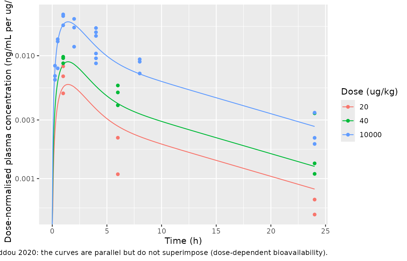

pk_pred_obs <- pk_obs |>
  dplyr::left_join(
    dplyr::select(sim_pk, dose_ugkg, time, pred = Cc),
    by = c("dose_ugkg", "time")
  )
stopifnot(!anyNA(pk_pred_obs$pred))
pk_fit <- pk_pred_obs |>
  dplyr::group_by(dose_ugkg) |>
  dplyr::summarise(gmr = exp(mean(log(pred / Cc))), .groups = "drop")
knitr::kable(
  pk_fit |> dplyr::rename("Dose (ug/kg)" = dose_ugkg, "Geometric mean predicted / observed" = gmr),
  digits = 2, caption = "Figure 4c: model predictions against the deposited plasma concentrations."
)

Figure 4c: model predictions against the deposited plasma concentrations.

Dose (ug/kg)	Geometric mean predicted / observed
20	1.21
40	0.83
10000	1.02

stopifnot(all(abs(log(pk_fit$gmr)) < log(1.5)))

PKNCA: the dose-dependent bioavailability

Bouhaddou 2020 reports no NCA table, so there is no published NCA to compare against. PKNCA is instead used to check the one PK feature that is easy to get wrong in translation, the saturable bioavailability. Dose / AUCinf is the apparent clearance CL/F; multiplied by the model’s F = D / (D50 + D) it must return CL = 117.66 mL/h at every dose, while the apparent clearance itself falls steeply with dose.

conc_pk <- sim_pk |>
  dplyr::filter(!is.na(Cc)) |>
  dplyr::mutate(treatment = paste(dose_ugkg, "ug/kg")) |>
  dplyr::select(id, time, Cc, treatment)
dose_pk <- ev_pk |>
  dplyr::filter(evid == 1) |>
  dplyr::mutate(treatment = paste(pk_doses[id], "ug/kg")) |>
  dplyr::select(id, time, amt, treatment)

o_conc <- PKNCA::PKNCAconc(conc_pk, Cc ~ time | treatment + id)
o_dose <- PKNCA::PKNCAdose(dose_pk, amt ~ time | treatment + id)
o_data <- PKNCA::PKNCAdata(
  o_conc, o_dose,
  intervals = data.frame(
    start = 0, end = Inf, cmax = TRUE, tmax = TRUE,
    aucinf.obs = TRUE, cl.obs = TRUE, half.life = TRUE
  )
)
nca_res <- PKNCA::pk.nca(o_data)

nca_wide <- as.data.frame(nca_res) |>
  dplyr::select(treatment, PPTESTCD, PPORRES) |>
  tidyr::pivot_wider(names_from = PPTESTCD, values_from = PPORRES) |>
  dplyr::mutate(
    dose_ng = as.numeric(sub(" ug/kg", "", treatment)) * 1e3 * 0.025,
    F = dose_ng / (1123.9 + dose_ng),
    cl_recovered = cl.obs * F
  ) |>
  dplyr::arrange(dose_ng)
knitr::kable(
  nca_wide |>
    dplyr::select(treatment, cmax, tmax, aucinf.obs, half.life, cl.obs, F, cl_recovered) |>
    dplyr::rename(
      "Dose" = treatment, "Cmax (ng/mL)" = cmax, "Tmax (h)" = tmax,
      "AUC0-inf (ng*h/mL)" = aucinf.obs, "t1/2 (h)" = half.life,
      "CL/F (mL/h)" = cl.obs, "F" = F, "CL/F x F (mL/h)" = cl_recovered
    ),
  digits = 3, caption = "PKNCA on the simulated single oral doses (0-168 h)."
)

PKNCA on the simulated single oral doses (0-168 h).

Dose	Cmax (ng/mL)	Tmax (h)	AUC0-inf (ng*h/mL)	t1/2 (h)	CL/F (mL/h)	F	CL/F x F (mL/h)
20 ug/kg	0.117	1.45	1.308	11.57	382.149	0.308	117.664
40 ug/kg	0.357	1.45	4.001	11.57	249.906	0.471	117.664
10000 ug/kg	188.725	1.45	2115.187	11.57	118.193	0.996	117.664

stopifnot(all(abs(nca_wide$cl_recovered / 117.66 - 1) < 0.02))

Figure 5 – predicted tumour growth under five regimens

tg_obs <- dplyr::bind_rows(
  tibble::tibble(
    arm = "Vehicle", day = c(7, 10, 14, 17, 21, 24, 28, 31, 35),
    vol = c(115.0, 122.9, 153.7, 224.7, 390.5, 644.0, 910.9, 1149.6, 1618.1)
  ),
  tibble::tibble(
    arm = "20 ug/kg QD 5on/2off", day = c(7, 10, 14, 17, 21, 24, 28, 31, 35),
    vol = c(75.7, 96.9, 153.1, 244.6, 438.2, 782.9, 1145.9, 1339.3, 1820.2)
  ),
  tibble::tibble(
    arm = "40 ug/kg QD 5on/2off", day = c(7, 10, 14, 17, 21, 24, 28, 31, 35),
    vol = c(76.9, 97.7, 154.5, 226.7, 323.5, 473.4, 682.4, 740.6, 1065.1)
  ),
  tibble::tibble(
    arm = "200 ug/kg weekly", day = c(6, 9, 13, 16, 21, 23, 27, 30),
    vol = c(79.4, 97.5, 146.6, 203.4, 459.1, 548.4, 864.6, 1162.6)
  ),
  tibble::tibble(
    arm = "400 ug/kg days 7, 16, 23", day = c(6, 9, 13, 16, 21, 23, 27, 30),
    vol = c(81.9, 98.2, 129.2, 147.0, 309.1, 424.0, 634.3, 807.9)
  )
) |>
  dplyr::mutate(arm = factor(arm, levels = levels(regimens$arm)))

ggplot(sim_vivo, aes(time / 24, tumor_vol)) +
  geom_line(colour = "steelblue", linewidth = 1) +
  geom_point(data = tg_obs, aes(day, vol), shape = 8) +
  facet_wrap(~arm, nrow = 1) +
  labs(
    x = "Time (days)", y = "Tumour volume (mm^3)",
    caption = "Replicates Figure 5b of Bouhaddou 2020. Line: model prediction; asterisks: observed means."
  )

sim_vivo |>
  dplyr::select(time, arm, Cc, roc, TE, grp) |>
  tidyr::pivot_longer(c(Cc, roc, TE, grp)) |>
  dplyr::mutate(name = factor(name, levels = c("Cc", "roc", "TE", "grp"))) |>
  ggplot(aes(time / 24, value, colour = arm)) +
  geom_line() +
  facet_wrap(~name, ncol = 1, scales = "free_y") +
  labs(
    x = "Time (days)", y = NULL, colour = NULL,
    caption = "Replicates Figure 5a: plasma (ng/mL), unbound tumour (nM), TE (%) and GRP mRNA."
  ) +
  theme(legend.position = "bottom")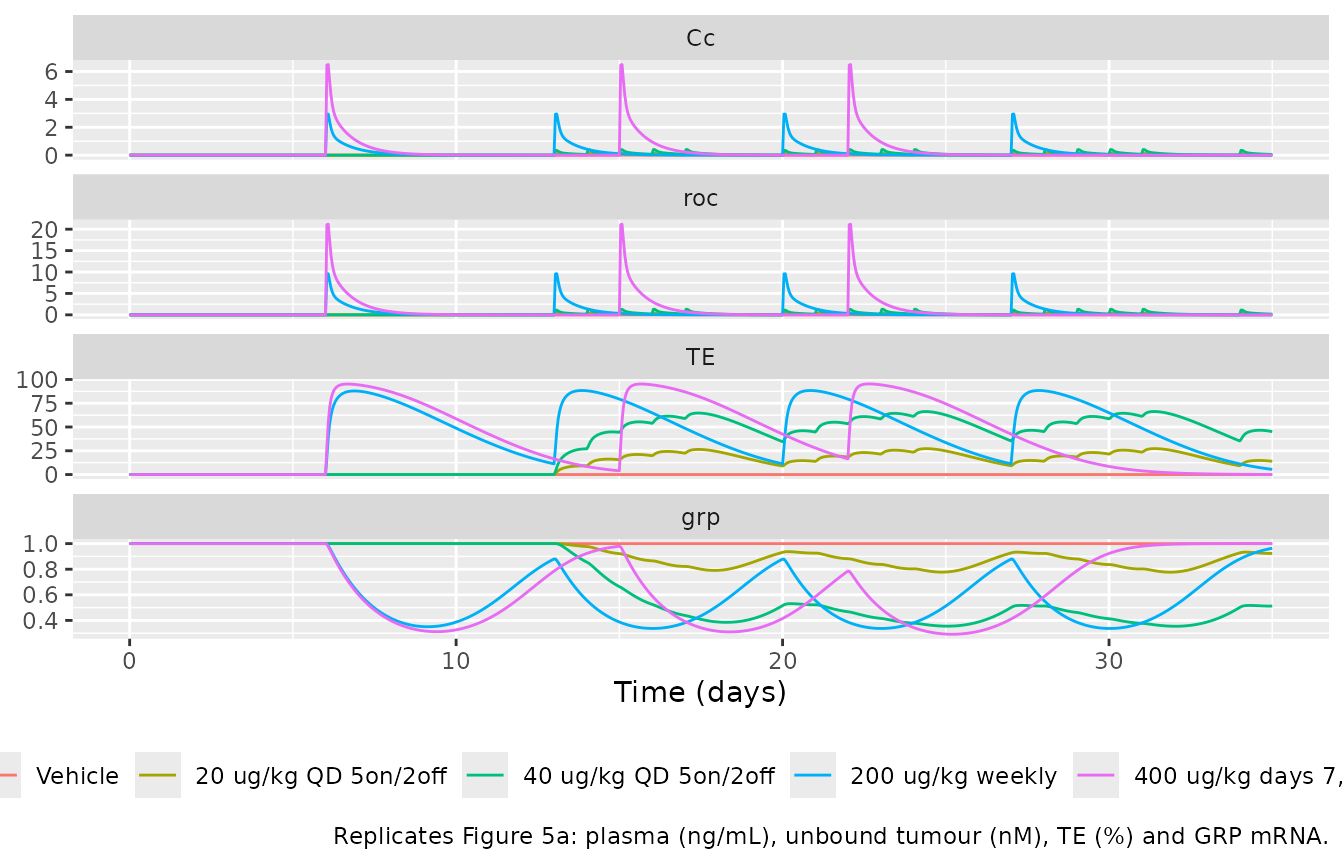

# Figure 5c: simulated versus observed at the observation times.
tg_cmp <- tg_obs |>
  dplyr::left_join(
    sim_vivo |> dplyr::mutate(day = time / 24) |> dplyr::select(arm, day, tumor_vol),
    by = c("arm", "day")
  )
stopifnot(!anyNA(tg_cmp$tumor_vol))

# Figure 5d: ratio of the areas under the tumour growth curves, computed with
# the authors' convention (Plot_TG_Predictions.m): the simulated area runs from
# day 0 to day 35 (day 30 for the two weekly arms), the observed area over the
# observed time points only.
trap <- function(x, y) sum(diff(x) * (utils::head(y, -1) + utils::tail(y, -1)) / 2)
sim_end <- c(35, 35, 35, 30, 30)
augic <- tg_cmp |>
  dplyr::group_by(arm) |>
  dplyr::summarise(auc_exp = trap(day, vol), .groups = "drop") |>
  dplyr::mutate(
    auc_sim = vapply(seq_along(arm), function(i) {
      s <- sim_vivo[sim_vivo$arm == arm[i] & sim_vivo$time <= sim_end[i] * 24, ]
      trap(s$time / 24, s$tumor_vol)
    }, numeric(1)),
    ratio = auc_sim / auc_exp,
    # Figure 5d bar heights, digitised by the maintainers (+/- 0.03).
    published = c(1.05, 0.91, 1.04, 0.78, 1.01)
  )
knitr::kable(
  augic |>
    dplyr::select(arm, ratio, published) |>
    dplyr::rename("Arm" = arm, "AUGIC ratio (this model)" = ratio, "AUGIC ratio, Fig. 5d" = published),
  digits = 2, caption = "Replicates Figure 5d: simulated / observed area under the tumour growth curve."
)

Replicates Figure 5d: simulated / observed area under the tumour growth curve.

Arm	AUGIC ratio (this model)	AUGIC ratio, Fig. 5d
Vehicle	1.05	1.05
20 ug/kg QD 5on/2off	0.90	0.91
40 ug/kg QD 5on/2off	1.04	1.04
200 ug/kg weekly	0.76	0.78
400 ug/kg days 7, 16, 23	1.00	1.01

stopifnot(
  # Reproduces the published bars; a wrong kP, dose conversion or PK
  # parameter moves these ratios by 0.1 or more.
  all(abs(augic$ratio - augic$published) < 0.06),
  # The drug effect is real: 40 ug/kg 5on/2off ends well below vehicle.
  tg_cmp$tumor_vol[tg_cmp$arm == "40 ug/kg QD 5on/2off" & tg_cmp$day == 35] <
    0.7 * tg_cmp$tumor_vol[tg_cmp$arm == "Vehicle" & tg_cmp$day == 35]
)

Assumptions and deviations

• Eq. 1 as printed is defective. It reads dX/dt = -ka * D/(D50 + D) * D, which does not balance against Eq. 2 (+ka * X). The deposited RunModelVivo.m implements a first-order depot, dX = -ka*X, and scales the administered amount once at dosing by D / (D50 + D) (Xup = (X0/(D50+X0))*X0). The model follows the code: a dose-dependent bioavailability f(depot) = podo(depot) / (D50 + podo(depot)), with the dose in ng. The reproduction gate above confirms the two are equivalent.
• kCL is a clearance, not a rate constant. Table S2 lists kCL = 117.66 1/h, but the code divides it by V (CL = CLml/V), and the parameter file names it CLml. It is encoded as CL = 117.66 mL/h (elimination rate constant 0.204 1/h).
• Dose units. D50 is “a.u.” in Table S2; the code applies it to the dose in ng after converting ug/kg with a fixed 0.025 kg mouse. Doses must therefore be entered in ng (ug/kg * 25).
• Unbound concentration in nM. Eq. 4 (ROc = CPL * fu) is completed with the ng/mL to nM conversion the code uses, 1000 / MW with MW = 230.4 g/mol (from the deposited parameter file; not printed in the paper).
• k50P in vivo. The Results say kP and k50P were re-estimated for the xenograft, but Table S2 lists k50P as “Same” and the deposited in vivo parameter file keeps 100000; the model uses 100000 (in mm^3 it is so large that growth is effectively exponential over 35 days).
• Point estimates vs intervals. Several Table S2 point estimates (e.g. vmax 0.03515 with 95% CI 0.0576-0.1914) lie outside the tabulated interval. The point estimates are the best-fit values also used in the deposited code (Value_BestEst); the intervals summarise the 25 accepted multistart parameter sets. The point estimates are used.
• Parameter-file label. In the deposited rateconstants_*_BEST.txt the sixth row (26.513) is labelled k50P; the code reads it positionally as the TE half-maximal constant K50, matching Table S2.
• abs() guards. The in vitro code wraps the state vector and 1 - GRP in abs(); both files keep abs(1 - GRP) (and the in vitro file abs(LSD1TOTAL - LSD1B)), which is inactive because GRP never exceeds 1 and bound LSD1 never exceeds the total, but prevents a round-off negative base being raised to the non-integer Hill powers.
• Alternative PK model not extracted. The nonlinear-clearance PK model (Eq. 21; ka 0.15 1/h, k12 2.02 1/h, k21 0.05 1/h, V 80.3 mL/kg, KM 27.2 ng/mL, Vmax 68.7 ng/(mL*h)) was a comparator the authors rejected in favour of nonlinear absorption (Figure S3); it is not part of the final model.
• No variability. The parameters were estimated by least squares on mean data, with no between-animal variability or residual-error model; both files are deterministic. The paper’s Figure S2 illustrates between-mouse spread by varying kP between 0.0022 and 0.0048 1/h, which users can reproduce by overriding lkp.
• Observed data. The observed points in the figures are the means in the authors’ deposited experimental_data.xlsx.
• No erratum or correction notice for this article was found (checked 2026-09-25).