Model and source
#> ℹ parameter labels from comments will be replaced by 'label()'Citation: Leding A. A. M., Bruinenberg P., Conradie A., Nedelman J., Lombardi A., Hickman D., Simonsson U. S. H. (2026). Population pharmacokinetics of TBAJ-587 and its main metabolites - Evaluation of different loading dose strategies and early dose selection. British Journal of Clinical Pharmacology 92(4):1058-1068. doi:10.1002/bcp.70333. Structure and all covariate / error equations transcribed from the final NONMEM control stream in Supporting Information Code S1; final parameter values from Table 1 (the Code S1 $THETA / $OMEGA records for the metabolite sub-models are initial estimates, not final ones).
Description: Joint parent + metabolite population PK model for the second-in-class diarylquinoline (DARQ) antitubercular TBAJ-587 and its two main metabolites M2 and M3 in healthy adult volunteers after single oral doses of 25-800 mg, followed to Day 126. TBAJ-587 has Savic 2007 analytical transit-compartment absorption (non-integer NN = 2.36 transit compartments feeding an absorption compartment that empties at ka) and three-compartment disposition; M3 has three-compartment and M2 two-compartment disposition, each formed in parallel from the parent central compartment. Both relative fractions metabolised are fixed at 1, so every metabolite clearance and volume is apparent relative to an unidentifiable true fraction metabolised, and each metabolite receives a formation flux equal to the parent’s whole elimination flux. Dose (a continuous covariate referenced to 200 mg) acts as a power function on parent clearance, on both fractions metabolised and on M2 clearance, and as an exponential function on ka; a high-calorie high-fat meal raises relative bioavailability and mean transit time and lowers both fractions metabolised. Residual variability is additive on the natural-log scale (lognormal) and estimated separately for each of the three analytes. Because no intravenous data were collected, all parent clearances and volumes are apparent oral values.
Article: https://doi.org/10.1002/bcp.70333
Supplement (Code S1 final NONMEM control stream, Tables S1-S2, Figures S1-S5): https://doi.org/10.1002/bcp.70333, Supporting Information
TBAJ-587 is a second-in-class diarylquinoline (DARQ) antitubercular, the class founded by bedaquiline. Leding 2026 describes the single-ascending-dose pharmacokinetics of TBAJ-587 and its two main metabolites, M2 and M3, and uses the model to pick a phase 2a dose and to ask whether a loading-dose period is worth its complexity.
The extraction is unusually well constrained because the supplement carries the complete final NONMEM control stream (Code S1). Two facts that only the control stream settles, and that would each have been a silent error if guessed from the paper body:
-
ktr = (NN + 1) / MTT, notNN / MTT. Code S1 statesKTR = (NN+1)/MTToutright. The paper body gives only “absorption transit compartments” and an estimatedNN, and the model estimates a separateka, which is the configuration in which the house convention of some groups isn / MTT. Guessing wrong shiftsktrby 42% here. -
The metabolite formation flux is not subtracted from the
parent. Code S1 keeps
-K20*A(2) = -CL/V2*A(2)inDADT(2)in full, and addsK25 = CL/V2*FM3andK28 = CL/V2*FM2as inflows to the two metabolite central compartments with no compensating loss. See “Parallel formation” below, which is the single most important thing to understand about this model.
One equally important trap runs the other way: the Code S1
$THETA and $OMEGA records for the metabolite
sub-models are initial estimates, not final ones.
CLM3 is 20.121 in Code S1 against 18.5 in Table 1, and
Q3 is 17.4191 against 9.09 – a factor of 1.9. The parent
block, by contrast, is FIX at exactly its Table 1 values.
So this extraction takes structure and every equation form from
Code S1, and every final value from Table 1.
Population
| Field | Value |
|---|---|
| species | human |
| n_subjects | 42 |
| n_studies | 1 |
| age_range | 18-64 years |
| bmi_range | 15.5-32.0 kg/m^2 |
| weight_range | minimum 50.0 kg (no upper bound or median reported) |
| disease_state | healthy volunteers |
| dose_range | single oral doses of 25, 50, 100, 200, 400 or 800 mg (n = 6, 4, 5, 8, 4 and 6 respectively), plus a nine-subject food-effect cohort dosed 200 mg with a high-calorie high-fat meal |
| trial | NCT04890535 Part 1; partially blinded, placebo-controlled, randomized single ascending dose with food-effect cohort |
| regions | Netherlands (single site; ethics approval ID NL73973.056.20) |
| notes | Leding 2026 Methods 2.1 and Results 3.1. Participants were male or female of non-childbearing potential; the sex split is not reported, so sex_female_pct is deliberately absent rather than guessed. 1929 observations were available for each of the three analytes, collected to Day 126; 29 of 42 subjects (69%) were sampled beyond Day 21 and 23 of those 29 (79%) beyond Day 112. Below-quantification-limit observations (LLOQ 1 ng/mL) made up 2%, 46% and 28% of records for TBAJ-587, M2 and M3 respectively; all parent BQL records were omitted, and metabolite BQL records were omitted except the first and last in the decreasing and ascending curve, which were set to LLOQ/2 (Leding 2026 Results 3.1). |
Forty-two healthy volunteers (male or female of non-childbearing
potential, 18-64 years, BMI 15.5-32.0 kg/m^2, minimum weight 50.0 kg)
received a single oral dose of TBAJ-587 in trial NCT04890535 Part 1 at
one Netherlands site. Six single-ascending-dose cohorts received 25, 50,
100, 200, 400 and 800 mg (n = 6, 4, 5, 8, 4 and 6), and a separate
nine-subject food-effect cohort received 200 mg with a high-calorie
high-fat meal. Plasma was sampled densely to 312 h, and 29 of 42
subjects (69%) were followed to Day 98 with 23 of those 29 (79%)
reaching Day 126 – follow-up that matters here because the terminal
half-life runs to months. 1929 observations were available for each of
the three analytes. The sex split is not reported in the paper, so
sex_female_pct is deliberately absent from the metadata
rather than guessed.
Note that the food effect is between-subject, not a crossover: the fed data come from nine subjects dosed only at 200 mg. Leding 2026 Discussion is explicit that the fed simulations therefore assume the dose dependence of apparent oral clearance, which was driven by the six fasted dose levels, carries over to the fed state.
Source trace
Per-parameter provenance is recorded as an in-file comment beside
each ini() entry in
inst/modeldb/specificDrugs/Leding_2026_tbaj587.R. Collected
here for review.
| Equation / parameter | Value | Source location |
|---|---|---|
Absorption input trin (Savic gamma density, Stirling
LNFAC) |
n/a | Code S1 $DES DADT(1); LNFAC
defined in $PK
|
ktr = (nn + 1) / mtt |
n/a | Code S1 $PK KTR = (NN+1)/MTT
|
f(depot) <- 0 |
n/a | Code S1 $PK F1 = 0
|
| Parent 3-cmt disposition | n/a | Code S1 $DES DADT(2)-DADT(4);
Figure 2; Results 3.2 |
| M3 3-cmt disposition | n/a | Code S1 $DES DADT(5)-DADT(7);
Figure 2; Results 3.2 |
| M2 2-cmt disposition | n/a | Code S1 $DES DADT(8)-DADT(9);
Figure 2; Results 3.2 |
Parallel formation K25, K28 (no parent
loss term) |
n/a | Code S1 $PK K25 = CL/V2*FM3,
K28 = CL/V2*FM2; Methods 2.2; Table 1 footnote a |
lfdepot (F fasted) |
1 (fixed) | Table 1 F fasted = 1 FIX; Code S1
$THETA(2)
|
lka |
0.0866 1/h | Table 1 ka, RSE 3.5% |
lcl |
5.40 L/h | Table 1 CL TBAJ-587, RSE 8.4% |
lvc |
88.2 L | Table 1 V C,TBAJ-587, RSE 6.8% |
lq / lvp
|
31.1 L/h / 1910 L | Table 1 Q P1,TBAJ-587, V P1,TBAJ-587
|
lq2 / lvp2
|
31.5 L/h / 22 500 L | Table 1 Q P2,TBAJ-587, V P2,TBAJ-587
|
lmtt |
0.837 h | Table 1 MTT fasted, RSE 4.5% |
lnn |
2.36 | Table 1 NN, RSE 8% |
e_fed_highfat_fdepot |
0.688 | Table 1 Fed state on F fasted; form from footnote
d |
e_dose_cl |
0.298 | Table 1 Dose covariate on CL TBAJ-587; power form from
footnote e |
e_dose_ka |
-0.000462 1/mg | Code S1 $THETA(13); Table 1 prints -0.00046 rounded;
exponential form from footnote f |
e_fed_highfat_mtt |
0.958 | Table 1 Fed state on MTT fasted; form from footnote
d |
lfm_m3 |
1 (fixed) | Table 1 f m,M3 = 1 FIX; Code S1
$THETA(15)
|
lcl_m3 / lvc_m3
|
18.5 L/h / 816 L | Table 1 CL M3, V C,M3
|
lq_m3 / lvp_m3
|
9.09 L/h / 1630 L | Table 1 Q P1,M3, V P1,M3
|
lq2_m3 / lvp2_m3
|
99.6 L/h / 3010 L | Table 1 Q P2,M3, V P2,M3
|
e_dose_fm_m3 |
-0.418 | Table 1 Dose covariate on f m,M3; power form from
footnote e |
e_fed_highfat_fm_m3 |
-0.479 | Table 1 Fed state on f m,M3; form from footnote d |
lfm_m2 |
1 (fixed) | Table 1 f m,M2 = 1 FIX; Code S1
$THETA(24)
|
lcl_m2 / lvc_m2
|
34.1 L/h / 247 L | Table 1 CL M2, V C,M2
|
lq_m2 / lvp_m2
|
174 L/h / 12 200 L | Table 1 Q P1,M2, V P1,M2
|
e_dose_fm_m2 |
-0.373 | Table 1 Dose covariate on f m,M2; power form from
footnote e |
e_fed_highfat_fm_m2 |
-0.547 | Table 1 Fed state on f m,M2; form from footnote d |
e_dose_cl_m2 |
0.146 | Table 1 Dose covariate on CL M2; power form from
footnote e |
| Parent IIV (7 etas) | see model file | Code S1 $OMEGA(1)-$OMEGA(7), all FIX; each
reproduces its Table 1 CV% |
| Metabolite IIV (5 etas) | see model file | Table 1 IIV CV% column, back-transformed as
omega^2 = log(1 + CV^2) (footnote c) |
expSd / expSd_m3 /
expSd_m2
|
0.1836 / 0.1954 / 0.1634 |
sqrt() of the Table 1 variances 0.0337 / 0.0382 /
0.0267; lnorm form from Code S1 $ERROR
|
Parallel formation with both fractions anchored at 1
This is the structural feature most likely to be mis-transcribed, so it is worth stating plainly. Methods 2.2 develops the metabolites “assuming parallel formation, using the fixed TBAJ-587 PK model and the assumption of f m, the fraction of TBAJ-587 cleared to metabolite, equalling one”, and Table 1 footnote a adds that for the metabolites “clearances and volumes are additionally relative to unknown fractions metabolized”.
In Code S1 that becomes: the parent’s total elimination is exactly
CL/V2, and each metabolite separately
receives an inflow of fm * CL/V2 * A(2) with
fm fixed at 1. The two fm values therefore
anchor at 1 rather than summing to 1, the metabolite amounts are not
mass-conserved against the parent, and each metabolite’s true
(unidentifiable) fraction metabolised is absorbed into its own apparent
clearance and volumes. The only estimated content of the two
fm parameters is their dose and food covariate effects,
plus IIV on fm_m2.
The tempting “repair” – subtracting the formation fluxes from the
parent to balance mass – would silently rescale every apparent
metabolite parameter in Table 1 and is wrong. The parameters are named
fm_m2 / fm_m3 (rather than the
clrat_<metab> canonical used when a formation arm
genuinely sits alongside the elimination arm) precisely because
the denominator each one divides is the parent’s whole clearance; see
the fm_<pathway> entry in
inst/references/parameter-names.md.
Units: a molar model validated against a mass-unit table
Leding 2026 fitted natural-log-transformed molar
concentrations: Code S1 $INPUT declares
AMT ; dose in nmol and
DV ; concentration in ln(nmol/L). The packaged model
therefore carries dosing = "nmol",
concentration = "nmol/L". But the dose covariates
act on the mg dose (DOSE ; dose in mg), which is why the
model needs the separate DOSE_TBAJ587_MG column, and why
neither quantity can be derived from the other: the paper
reports no molecular weight.
That is not an obstacle for the parent, because the molecular weight
cancels. Writing M for the parent molecular weight, a
D mg dose is D * 1e6 / M nmol, concentrations
scale linearly with the dosed amount, and converting back to mass units
multiplies by M * 1e-6 – so any mass-unit exposure is
proportional to D with M absent. Equivalently,
dosing the numeric mg value into the nmol slot returns parent
concentrations directly in mg/L. The chunk below verifies that
invariance numerically rather than asserting it, then uses the resulting
scaffold throughout.
mod <- rxode2::zeroRe(readModelDb("Leding_2026_tbaj587"))
#> ℹ parameter labels from comments will be replaced by 'label()'

# Helper: build a dosing + observation event table. Observation rows carry
# cmt = "central" (an ODE STATE, never the observable name "Cc") plus
# dvid = 1L to nominate an endpoint in this three-output model.
make_events <- function(dose_mg, dose_times, obs_times, fed, amt = dose_mg) {
  dos <- data.frame(time = dose_times, amt = amt, evid = 1L,
                    cmt = "depot", dvid = NA_integer_)
  obs <- data.frame(time = obs_times, amt = NA_real_, evid = 0L,
                    cmt = "central", dvid = 1L)
  ev <- rbind(dos, obs)
  ev <- ev[order(ev$time, ev$evid == 0L), ]
  ev$DOSE_TBAJ587_MG <- dose_mg
  ev$FED_HIGHFAT <- fed
  ev$id <- 1L
  ev
}

trapz <- function(x, y) sum(diff(x) * (utils::head(y, -1) + utils::tail(y, -1)) / 2)

# Observation grid for the single-dose AUCinf work below. It must be FINE
# through absorption and distribution and may be coarse through the
# months-long terminal phase: a uniform 24 h grid understates AUC by ~0.3%
# because Tmax is around 4 h, which is enough to break a 1e-3 mass-balance
# gate for reasons that have nothing to do with the model.
auc_grid <- unique(c(seq(0, 24, by = 0.05),
                     seq(24, 312, by = 1),
                     seq(312, 24 * 365 * 8, by = 24)))

# Solve a single 200 mg fasted dose under two assumed molecular weights and
# convert each AUC back to mass units.
auc_mass <- vapply(c(500, 1000), function(MW) {
  ev <- make_events(200, 0, auc_grid, fed = 0, amt = 200 * 1e6 / MW)
  s <- as.data.frame(rxode2::rxSolve(mod, ev, atol = 1e-12, rtol = 1e-10,
                                     maxsteps = 1e6))
  s <- s[!is.na(s$Cc), ]
  trapz(s$time, s$Cc) * MW * 1e-6           # h*nmol/L -> h*mg/L
}, numeric(1))
#> ℹ omega/sigma items treated as zero: 'etalka', 'etalfdepot', 'etalcl', 'etalvc', 'etalvp', 'etalvp2', 'etalmtt', 'etalcl_m3', 'etalvc_m3', 'etalfm_m2', 'etalvc_m2', 'etalvp_m2'
#> ℹ omega/sigma items treated as zero: 'etalka', 'etalfdepot', 'etalcl', 'etalvc', 'etalvp', 'etalvp2', 'etalmtt', 'etalcl_m3', 'etalvc_m3', 'etalfm_m2', 'etalvc_m2', 'etalvp_m2'

# Deterministic (zeroRe) quantities, so this can be asserted tightly.
stopifnot(abs(auc_mass[1] / auc_mass[2] - 1) < 1e-6)
sprintf("AUCinf in h*mg/L at MW = 500 and 1000 g/mol: %.4f vs %.4f (ratio %.9f)",
        auc_mass[1], auc_mass[2], auc_mass[1] / auc_mass[2])
#> [1] "AUCinf in h*mg/L at MW = 500 and 1000 g/mol: 38.3621 vs 38.3621 (ratio 1.000000000)"
For the metabolites the cancellation is incomplete:
a metabolite’s mass-unit exposure carries the ratio
MW_metabolite / MW_parent. The paper states that ratio only
qualitatively, and only for M3 – Discussion: “the difference in
molecular weight between TBAJ-587 and M3 is only 2%”. The “Recovering
the molecular-weight ratios” section below turns that into a
quantitative check.
Throughout the rest of this vignette the dose amount is the numeric
mg value, so Cc reads directly in mg/L and
Cc_m3 / Cc_m2 read in parent-molar-
equivalent mg/L.
Structural verification
Stirling approximation in the absorption normaliser
Code S1 normalises the Savic gamma density with a Stirling
approximation to log(NN!) rather than the exact
lgamma(NN+1):
LNFAC = LOG(2.5066)+(NN+0.5)*LOG(NN)-NNAt NN = 2.36 that understates log(NN!), so
the input rate integrates to slightly more than
F * dose. The model file reproduces the approximation
verbatim, because it is the expression against which every Table 1 value
– CL above all – was estimated. The factor is measured here
so the mass-balance gate below has an exact target instead of a
fudge.
nn_hat  <- 2.36
lnfac   <- log(2.5066) + (nn_hat + 0.5) * log(nn_hat) - nn_hat
stirling_factor <- exp(lgamma(nn_hat + 1) - lnfac)
sprintf("Stirling LNFAC = %.6f vs exact lgamma(NN+1) = %.6f; input inflated by %.4f%%",
        lnfac, lgamma(nn_hat + 1), 100 * (stirling_factor - 1))
#> [1] "Stirling LNFAC = 1.014699 vs exact lgamma(NN+1) = 1.049820; input inflated by 3.5744%"
Mass balance on all three analytes
This is the load-bearing gate. The f(depot) <- 0
idiom that a NONMEM F1 = 0 requires can, for some models,
make the whole d/dt(depot) right-hand side evaluate to zero
– a flat-zero solve that produces no error and no
NA, and that ratio-based checks cannot detect
because they divide one zero by another. The only check that catches it
is absolute mass balance, and it also catches the opposite failure of a
dose arriving twice.
At steady state after a single dose, cl * AUCinf must
equal dose * F * stirling_factor for the parent. For each
metabolite, whose inflow is fm * cl * Cc with
fm = 1 at the 200 mg fasted reference,
cl_metab * AUCinf_metab must equal the same quantity.
ev_mb <- make_events(200, 0, auc_grid, fed = 0)
s_mb <- as.data.frame(rxode2::rxSolve(mod, ev_mb, atol = 1e-12, rtol = 1e-10,
                                      maxsteps = 1e6))
#> ℹ omega/sigma items treated as zero: 'etalka', 'etalfdepot', 'etalcl', 'etalvc', 'etalvp', 'etalvp2', 'etalmtt', 'etalcl_m3', 'etalvc_m3', 'etalfm_m2', 'etalvc_m2', 'etalvp_m2'
s_mb <- s_mb[!is.na(s_mb$Cc), ]

# Apparent clearances at the 200 mg fasted reference: every dose factor is
# (200/200)^x = 1 and every fed factor is 1, so these are the Table 1 values.
target <- 200 * 1 * stirling_factor
mb <- tibble::tibble(
  Analyte = c("TBAJ-587", "M3", "M2"),
  `cl * AUCinf` = c(5.40 * trapz(s_mb$time, s_mb$Cc),
                    18.5 * trapz(s_mb$time, s_mb$Cc_m3),
                    34.1 * trapz(s_mb$time, s_mb$Cc_m2)),
  Target = target
) |>
  dplyr::mutate(Ratio = `cl * AUCinf` / Target)

# Deterministic; realised deviation is ~3e-5 on all three analytes, so 1e-3
# leaves room only for the trapezoid grid and Code S1's own 1e-5 log-guard
# offsets while still going red on a zeroed depot (ratio 0), a doubled dose
# (ratio 2), or a compensating parent loss term (metabolite ratios halve).
stopifnot(all(abs(mb$Ratio - 1) < 1e-3))

# Each analyte actually rises (the flat-zero failure mode this gate exists to
# catch), and nothing decays into negative solver noise over the 8-year
# horizon. Note Cc is exactly 0 at t = 0 by construction: f(depot) <- 0 means
# the dose never lands as a bolus, so `> 0` would fail on the pre-dose row.
stopifnot(max(s_mb$Cc) > 0, max(s_mb$Cc_m3) > 0, max(s_mb$Cc_m2) > 0)
stopifnot(all(s_mb$Cc >= 0), all(s_mb$Cc_m3 >= 0), all(s_mb$Cc_m2 >= 0))
knitr::kable(mb, digits = c(0, 4, 4, 6),
caption = "Mass balance after a single 200 mg fasted dose.")| Analyte | cl * AUCinf | Target | Ratio |
|---|---|---|---|
| TBAJ-587 | 207.1552 | 207.1489 | 1.000030 |
| M3 | 207.1539 | 207.1489 | 1.000024 |
| M2 | 207.1524 | 207.1489 | 1.000017 |
The transit chain is live and ktr = (NN+1)/MTT is
load-bearing
A model whose ODE chain had been silently discarded, or whose
absorption input had collapsed, would still reproduce AUC exactly – AUC
is dose * F / CL whatever the absorption shape. Tmax is the
discriminator. Quadrupling MTT on a
single-dose solve must move it materially; on a
multiple-dose event table Tmax would pin to the next dose time under any
reading and the check would be vacuous.
tmax_at <- function(mtt_factor) {
  m <- mod |> rxode2::ini(lmtt = log(0.837 * mtt_factor))
  ev <- make_events(200, 0, seq(0, 72, by = 0.05), fed = 0)
  s <- as.data.frame(rxode2::rxSolve(m, ev))
  s <- s[!is.na(s$Cc), ]
  s$time[which.max(s$Cc)]
}
tmax_1x <- tmax_at(1)
#> ℹ change initial estimate of `lmtt` to `-0.177931208492662`
#> ℹ omega/sigma items treated as zero: 'etalka', 'etalfdepot', 'etalcl', 'etalvc', 'etalvp', 'etalvp2', 'etalmtt', 'etalcl_m3', 'etalvc_m3', 'etalfm_m2', 'etalvc_m2', 'etalvp_m2'
tmax_4x <- tmax_at(4)
#> ℹ change initial estimate of `lmtt` to `1.20836315262723`
#> ℹ omega/sigma items treated as zero: 'etalka', 'etalfdepot', 'etalcl', 'etalvc', 'etalvp', 'etalvp2', 'etalmtt', 'etalcl_m3', 'etalvc_m3', 'etalfm_m2', 'etalvc_m2', 'etalvp_m2'
stopifnot(tmax_4x - tmax_1x > 2)
sprintf("Tmax at MTT 0.837 h = %.2f h; at 3.348 h = %.2f h (shift %.2f h)",
        tmax_1x, tmax_4x, tmax_4x - tmax_1x)
#> [1] "Tmax at MTT 0.837 h = 4.25 h; at 3.348 h = 7.75 h (shift 3.50 h)"
Replicating Table S2: AUC0-24h at the end of week 4
Table S2 is the paper’s quantitative prediction table:
AUC0-24h at the end of week 4 of once-daily dosing in the
fed state, without a loading period, at each of the six studied dose
levels, for all three analytes. It is simulated here with typical values
(zeroRe), which is what a “predicted” typical exposure
table calls for, and the interval AUC comes from PKNCA
over the final dosing interval.
doses <- c(25, 50, 100, 200, 400, 800)
tau <- 24
start_ss <- 27 * tau        # start of the 28th (final) dosing interval
end_ss   <- 28 * tau

sim_s2 <- lapply(doses, function(D) {
  ev <- make_events(D, seq(0, start_ss, by = tau),
                    seq(start_ss, end_ss, by = 0.25), fed = 1)
  s <- as.data.frame(rxode2::rxSolve(mod, ev, atol = 1e-10, rtol = 1e-8,
                                     maxsteps = 1e6))
  s$treatment <- paste(D, "mg")
  s$amt_mg <- D
  s
}) |>
  dplyr::bind_rows() |>
  dplyr::filter(!is.na(Cc))
#> ℹ omega/sigma items treated as zero: 'etalka', 'etalfdepot', 'etalcl', 'etalvc', 'etalvp', 'etalvp2', 'etalmtt', 'etalcl_m3', 'etalvc_m3', 'etalfm_m2', 'etalvc_m2', 'etalvp_m2'
#> ℹ omega/sigma items treated as zero: 'etalka', 'etalfdepot', 'etalcl', 'etalvc', 'etalvp', 'etalvp2', 'etalmtt', 'etalcl_m3', 'etalvc_m3', 'etalfm_m2', 'etalvc_m2', 'etalvp_m2'
#> ℹ omega/sigma items treated as zero: 'etalka', 'etalfdepot', 'etalcl', 'etalvc', 'etalvp', 'etalvp2', 'etalmtt', 'etalcl_m3', 'etalvc_m3', 'etalfm_m2', 'etalvc_m2', 'etalvp_m2'
#> ℹ omega/sigma items treated as zero: 'etalka', 'etalfdepot', 'etalcl', 'etalvc', 'etalvp', 'etalvp2', 'etalmtt', 'etalcl_m3', 'etalvc_m3', 'etalfm_m2', 'etalvc_m2', 'etalvp_m2'
#> ℹ omega/sigma items treated as zero: 'etalka', 'etalfdepot', 'etalcl', 'etalvc', 'etalvp', 'etalvp2', 'etalmtt', 'etalcl_m3', 'etalvc_m3', 'etalfm_m2', 'etalvc_m2', 'etalvp_m2'
#> ℹ omega/sigma items treated as zero: 'etalka', 'etalfdepot', 'etalcl', 'etalvc', 'etalvp', 'etalvp2', 'etalmtt', 'etalcl_m3', 'etalvc_m3', 'etalfm_m2', 'etalvc_m2', 'etalvp_m2'

# One PKNCA pass per analyte (multi-output model). auclast over the final
# interval is AUC0-24h at the end of week 4.
auc_week4 <- function(conc_col) {
  nca_in <- sim_s2 |>
    dplyr::select(treatment, time, dplyr::all_of(conc_col)) |>
    dplyr::rename(Cc = dplyr::all_of(conc_col)) |>
    dplyr::mutate(id = 1L)

  dose_df <- sim_s2 |>
    dplyr::distinct(treatment, amt_mg) |>
    tidyr::crossing(time = seq(0, start_ss, by = tau)) |>
    dplyr::mutate(id = 1L, amt = amt_mg) |>
    dplyr::select(id, time, amt, treatment)

  conc_obj <- PKNCA::PKNCAconc(nca_in, Cc ~ time | treatment + id,
                               concu = "mg/L", timeu = "h")
  dose_obj <- PKNCA::PKNCAdose(dose_df, amt ~ time | treatment + id,
                               doseu = "mg")
  intervals <- data.frame(start = start_ss, end = end_ss,
                          auclast = TRUE, cmax = TRUE, cmin = TRUE, cav = TRUE)
  res <- PKNCA::pk.nca(PKNCA::PKNCAdata(conc_obj, dose_obj,
                                        intervals = intervals))
  as.data.frame(res$result)
}

nca_p  <- auc_week4("Cc")
nca_m3 <- auc_week4("Cc_m3")
nca_m2 <- auc_week4("Cc_m2")

nca_value <- function(df, param) {
  out <- df[df$PPTESTCD == param, c("treatment", "PPORRES")]
  # Guard against a silently-empty lookup (all(logical(0)) is TRUE).
  stopifnot(nrow(out) == length(doses))
  out$PPORRES[match(paste(doses, "mg"), out$treatment)]
}

published <- tibble::tibble(
  dose   = doses,
  p_pub  = c(2.08, 4.05, 7.83, 15.1, 28.8, 54.4),
  m3_pub = c(0.296, 0.532, 0.951, 1.69, 2.98, 5.21),
  m2_pub = c(0.139, 0.244, 0.425, 0.734, 1.25, 2.12)
)

cmp_s2 <- published |>
  dplyr::mutate(
    p_sim  = nca_value(nca_p,  "auclast"),
    m3_sim = nca_value(nca_m3, "auclast"),
    m2_sim = nca_value(nca_m2, "auclast"),
    p_pct  = 100 * (p_sim  - p_pub)  / p_pub,
    m3_pct = 100 * (m3_sim - m3_pub) / m3_pub,
    m2_pct = 100 * (m2_sim - m2_pub) / m2_pub
  )

cmp_s2 |>
  dplyr::select(dose, p_pub, p_sim, p_pct, m3_pub, m3_sim, m3_pct,
                m2_pub, m2_sim, m2_pct) |>
  dplyr::rename(
    "Dose (mg)"          = dose,
    "Parent pub"         = p_pub,
    "Parent sim"         = p_sim,
    "Parent %diff"       = p_pct,
    "M3 pub"             = m3_pub,
    "M3 sim"             = m3_sim,
    "M3 %diff"           = m3_pct,
    "M2 pub"             = m2_pub,
    "M2 sim"             = m2_sim,
    "M2 %diff"           = m2_pct
  ) |>
  knitr::kable(
    digits = 3,
    caption = paste(
      "AUC0-24h (h*mg/L) at the end of week 4, once-daily fed dosing, no",
      "loading period. Published values from Leding 2026 Table S2; simulated",
      "values are typical-value (zeroRe) PKNCA auclast over the final dosing",
      "interval. Metabolite simulated values are in parent-molar-equivalent",
      "mass units, so their offset is the molecular-weight ratio (see below)."
    )
)| Dose (mg) | Parent pub | Parent sim | Parent %diff | M3 pub | M3 sim | M3 %diff | M2 pub | M2 sim | M2 %diff |
|---|---|---|---|---|---|---|---|---|---|
| 25 | 2.08 | 2.078 | -0.078 | 0.296 | 0.303 | 2.474 | 0.139 | 0.142 | 1.981 |
| 50 | 4.05 | 4.046 | -0.100 | 0.532 | 0.545 | 2.403 | 0.244 | 0.249 | 2.187 |
| 100 | 7.83 | 7.833 | 0.043 | 0.951 | 0.974 | 2.374 | 0.425 | 0.435 | 2.324 |
| 200 | 15.10 | 15.069 | -0.206 | 1.690 | 1.729 | 2.336 | 0.734 | 0.751 | 2.360 |
| 400 | 28.80 | 28.769 | -0.106 | 2.980 | 3.050 | 2.360 | 1.250 | 1.284 | 2.731 |
| 800 | 54.40 | 54.435 | 0.064 | 5.210 | 5.332 | 2.342 | 2.120 | 2.167 | 2.238 |
The parent reproduces Table S2 to a median absolute
difference of 0.09% across a 32-fold dose range. That is a demanding
joint test: it exercises the Stirling normaliser, the
(NN+1)/MTT transit rate, the power dose effect on
clearance, both high-fat meal effects, and 28 days of accumulation with
a months-long terminal half-life. A mis-transcribed clearance, dose
reference or unit would move it by tens of percent.
# Deterministic typical-value quantities, so these are tight by design.
stopifnot(max(abs(cmp_s2$p_pct)) < 1)
# Metabolites sit ~2.3% high purely from the molar-to-mass conversion; bound
# them well inside the 20% that would indicate a structural error.
stopifnot(max(abs(cmp_s2$m3_pct)) < 5, max(abs(cmp_s2$m2_pct)) < 5)
Recovering the molecular-weight ratios
The metabolite columns are offset by a nearly constant factor across
all six dose levels. A structural error would not behave that
way – it would grow or shrink with dose, because the dose covariates on
fm_m2, fm_m3 and cl_m2 are what
make metabolite exposure dose-dependent. A constant multiplicative
offset is the signature of a unit conversion, and the only conversion
left unspecified is the molar-to-mass one.
Inverting it recovers each metabolite’s molecular weight relative to the parent’s. For M3 the paper gives an independent check on the answer.
mw_ratio <- tibble::tibble(
  Metabolite = c("M3", "M2"),
  `Implied MW ratio to parent` = c(median(cmp_s2$m3_pub / cmp_s2$m3_sim),
                                   median(cmp_s2$m2_pub / cmp_s2$m2_sim)),
  `Spread across the 6 doses` = c(
    diff(range(cmp_s2$m3_pub / cmp_s2$m3_sim)),
    diff(range(cmp_s2$m2_pub / cmp_s2$m2_sim))
  )
)
mw_ratio$`Implied MW difference` <-
  sprintf("%.1f%%", 100 * (1 - mw_ratio$`Implied MW ratio to parent`))

# The offset must be essentially dose-independent for the unit-conversion
# reading to hold at all; a structural error would not be.
stopifnot(all(mw_ratio$`Spread across the 6 doses` < 0.01))
# Leding 2026 Discussion: "the difference in molecular weight between TBAJ-587
# and M3 is only 2%". Recovered independently from Table S2.
stopifnot(abs(1 - mw_ratio$`Implied MW ratio to parent`[1]) < 0.04)

knitr::kable(mw_ratio, digits = 4, caption = paste(
  "Metabolite/parent molecular-weight ratios recovered by inverting the",
  "molar-to-mass conversion implied by Table S2. The M3 value is an",
  "independent check on the paper's stated 2% difference."
))| Metabolite | Implied MW ratio to parent | Spread across the 6 doses | Implied MW difference |
|---|---|---|---|
| M3 | 0.9769 | 0.0013 | 2.3% |
| M2 | 0.9777 | 0.0072 | 2.2% |
M3’s recovered ratio of 0.977 is a 2.3% molecular-weight difference, matching the paper’s stated “only 2%” and confirming both that the metabolite offset is a unit conversion rather than a transcription error and that the M3 sub-model is correct. M2’s ratio is recovered at 0.978; the paper never states it, so this is a prediction rather than a confirmation.
Dose proportionality and metabolite abundance
Results 3.2: “Increases in predicted exposure were approximately dose-proportional for TBAJ-587, slightly less so for M2 and M3.” Results 3.1: “Abundance in plasma was in decreasing order: TBAJ-587, M3 and M2.”
prop <- cmp_s2 |>
  dplyr::transmute(
    dose,
    `TBAJ-587` = (p_sim  / dose) / (p_sim[dose == 200]  / 200),
    M3         = (m3_sim / dose) / (m3_sim[dose == 200] / 200),
    M2         = (m2_sim / dose) / (m2_sim[dose == 200] / 200)
  )

# Parent is closer to proportional (normalised AUC flatter) than either
# metabolite: a deterministic ordering of three deterministic spreads.
span <- function(x) diff(range(x))
stopifnot(span(prop$`TBAJ-587`) < span(prop$M3),
          span(prop$`TBAJ-587`) < span(prop$M2))
# Parent stays within 25% of proportional across a 32-fold dose range.
stopifnot(span(prop$`TBAJ-587`) < 0.25)

# Abundance order, typical values at 200 mg fed.
ord <- cmp_s2[cmp_s2$dose == 200, ]
stopifnot(ord$p_sim > ord$m3_sim, ord$m3_sim > ord$m2_sim)

prop |>
  dplyr::rename("Dose (mg)" = dose) |>
  knitr::kable(digits = 3, caption = paste(
    "Dose-normalised AUC0-24h at the end of week 4, referenced to 200 mg.",
    "1.0 would be exact dose proportionality."
))| Dose (mg) | TBAJ-587 | M3 | M2 |
|---|---|---|---|
| 25 | 1.103 | 1.403 | 1.509 |
| 50 | 1.074 | 1.260 | 1.327 |
| 100 | 1.040 | 1.126 | 1.158 |
| 200 | 1.000 | 1.000 | 1.000 |
| 400 | 0.955 | 0.882 | 0.855 |
| 800 | 0.903 | 0.771 | 0.721 |
sim_s2 |>
  dplyr::filter(treatment == "200 mg") |>
  dplyr::select(time, `TBAJ-587` = Cc, M3 = Cc_m3, M2 = Cc_m2) |>
  tidyr::pivot_longer(-time, names_to = "Analyte", values_to = "conc") |>
  ggplot(aes(time - start_ss, conc, colour = Analyte)) +
  geom_line(linewidth = 0.8) +
  scale_y_log10() +
  labs(x = "Time within the final dosing interval (h)",
       y = "Concentration (mg/L, metabolites parent-molar-equivalent)",
       title = "Analyte abundance at 200 mg once daily, end of week 4",
       caption = paste("Reproduces the ordering reported in Leding 2026",
                       "Results 3.1 and visible in Figure 1."))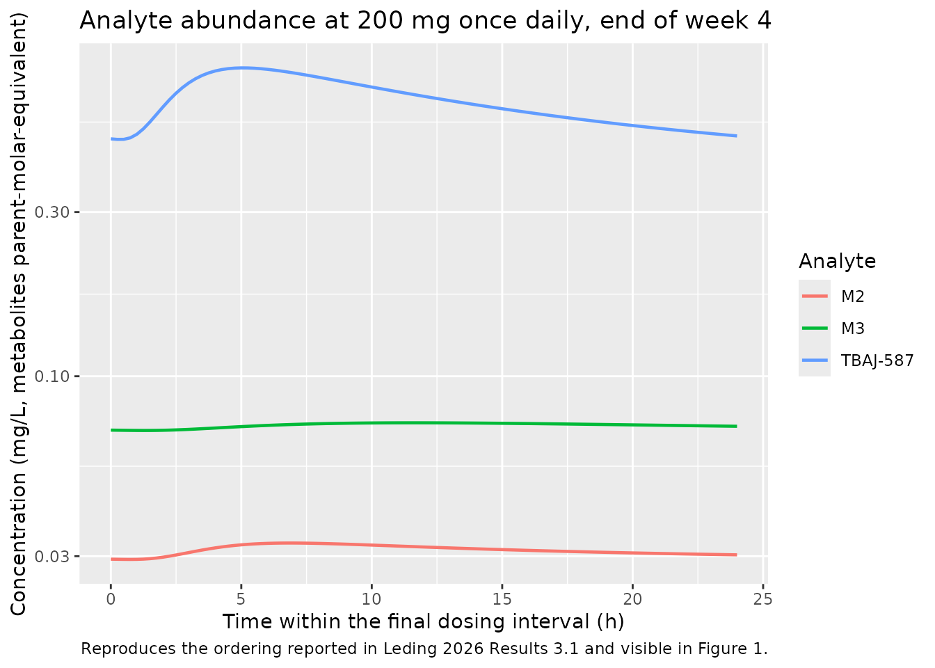
Terminal half-life across the dose range
Results 3.2: “The terminal half-life was predicted to range from 3.5 to 9.0 months for the explored dose range.” Because apparent clearance rises with dose, the shortest half-life belongs to the highest dose. This is an independent check – nothing in the transcription was fitted to it.
term_thalf <- function(D) {
  ev <- make_events(D, 0, seq(0, 24 * 365 * 3, by = 24), fed = 0)
  s <- as.data.frame(rxode2::rxSolve(mod, ev, atol = 1e-12, rtol = 1e-10,
                                     maxsteps = 1e6))
  s <- s[!is.na(s$Cc) & s$Cc > 0, ]
  # Fit the slope well after absorption and distribution have died away, so
  # this is the terminal phase and not a washout transient.
  # Keep Cc >= 1e-6 * max(Cc) so the fit never reaches the solver-noise tail.
  tl <- s[s$time > 24 * 365 * 1.5 & s$Cc >= 1e-6 * max(s$Cc), ]
  k <- -stats::coef(stats::lm(log(Cc) ~ time, data = tl))[["time"]]
  log(2) / k / (24 * 30.44)
}
thalf <- tibble::tibble(
  `Dose (mg)` = c(25, 800),
  `Terminal half-life (months)` = vapply(c(25, 800), term_thalf, numeric(1))
)
#> ℹ omega/sigma items treated as zero: 'etalka', 'etalfdepot', 'etalcl', 'etalvc', 'etalvp', 'etalvp2', 'etalmtt', 'etalcl_m3', 'etalvc_m3', 'etalfm_m2', 'etalvc_m2', 'etalvp_m2'
#> ℹ omega/sigma items treated as zero: 'etalka', 'etalfdepot', 'etalcl', 'etalvc', 'etalvp', 'etalvp2', 'etalmtt', 'etalcl_m3', 'etalvc_m3', 'etalfm_m2', 'etalvc_m2', 'etalvp_m2'

# Published range 3.5-9.0 months over 25-800 mg. Deterministic; 1 month of
# tolerance absorbs the choice of tail window without admitting a wrong model.
stopifnot(abs(thalf$`Terminal half-life (months)`[1] - 9.0) < 1,
          abs(thalf$`Terminal half-life (months)`[2] - 3.5) < 1)
stopifnot(thalf$`Terminal half-life (months)`[1] >
            thalf$`Terminal half-life (months)`[2])
knitr::kable(thalf, digits = 2, caption = paste(
  "Terminal half-life at the extremes of the studied dose range, single",
  "fasted dose. Leding 2026 Results 3.2 reports 3.5 to 9.0 months."
))| Dose (mg) | Terminal half-life (months) |
|---|---|
| 25 | 8.63 |
| 800 | 3.48 |
Replicating Figure 3: loading doses and time to steady state
Leding 2026 explored 2-week loading periods at 2:1, 3:1 and 4:1 to
the maintenance dose, followed by 10 weeks of maintenance dosing, and
compared them against no loading period. Cavg is
AUC0-24h / 24 (Equation 5).
build_regimen <- function(maint, ratio, weeks = 12) {
  ld_days <- if (ratio > 1) 14 else 0
  day <- seq(0, weeks * 7 - 1)
  dose_mg <- ifelse(day < ld_days, maint * ratio, maint)
  dos <- data.frame(time = day * 24, amt = dose_mg, evid = 1L, cmt = "depot",
                    dvid = NA_integer_, DOSE_TBAJ587_MG = dose_mg)
  ot <- seq(0, weeks * 7 * 24, by = 2)
  obs <- data.frame(
    time = ot, amt = NA_real_, evid = 0L, cmt = "central", dvid = 1L,
    # The dose covariate is time-varying here: it takes the loading mg dose
    # during the loading period and the maintenance mg dose thereafter.
    DOSE_TBAJ587_MG = stats::approx(dos$time, dos$DOSE_TBAJ587_MG, ot,
                                    method = "constant", rule = 2)$y
  )
  ev <- rbind(dos, obs)
  ev <- ev[order(ev$time, ev$evid == 0L), ]
  ev$FED_HIGHFAT <- 1
  ev$id <- 1L
  ev$regimen <- if (ratio > 1) paste0(ratio, "x loading") else "no loading"
  ev
}

cavg_on_day <- function(s, day) {
  w <- s[s$time >= (day - 1) * 24 & s$time <= day * 24, ]
  trapz(w$time, w$Cc) / 24
}

regimens <- c(1, 2, 3, 4)
sim_load <- lapply(regimens, function(r) {
  ev <- build_regimen(100, r)
  s <- as.data.frame(rxode2::rxSolve(mod, ev, keep = "regimen",
                                     atol = 1e-10, rtol = 1e-8, maxsteps = 1e6))
  s <- s[!is.na(s$Cc), ]
  s$ratio <- r
  s
}) |>
  dplyr::bind_rows()
#> ℹ omega/sigma items treated as zero: 'etalka', 'etalfdepot', 'etalcl', 'etalvc', 'etalvp', 'etalvp2', 'etalmtt', 'etalcl_m3', 'etalvc_m3', 'etalfm_m2', 'etalvc_m2', 'etalvp_m2'
#> ℹ omega/sigma items treated as zero: 'etalka', 'etalfdepot', 'etalcl', 'etalvc', 'etalvp', 'etalvp2', 'etalmtt', 'etalcl_m3', 'etalvc_m3', 'etalfm_m2', 'etalvc_m2', 'etalvp_m2'
#> ℹ omega/sigma items treated as zero: 'etalka', 'etalfdepot', 'etalcl', 'etalvc', 'etalvp', 'etalvp2', 'etalmtt', 'etalcl_m3', 'etalvc_m3', 'etalfm_m2', 'etalvc_m2', 'etalvp_m2'
#> ℹ omega/sigma items treated as zero: 'etalka', 'etalfdepot', 'etalcl', 'etalvc', 'etalvp', 'etalvp2', 'etalmtt', 'etalcl_m3', 'etalvc_m3', 'etalfm_m2', 'etalvc_m2', 'etalvp_m2'

cavg_tab <- lapply(regimens, function(r) {
  s <- sim_load[sim_load$ratio == r, ]
  tibble::tibble(ratio = r,
                 regimen = if (r > 1) paste0(r, "x loading") else "no loading",
                 d14 = cavg_on_day(s, 14), d28 = cavg_on_day(s, 28),
                 d56 = cavg_on_day(s, 56), d84 = cavg_on_day(s, 84))
}) |>
  dplyr::bind_rows()

sim_load |>
  ggplot(aes(time / 24, Cc, colour = regimen)) +
  geom_line(linewidth = 0.7) +
  geom_vline(xintercept = 14, linetype = "dotted") +
  labs(x = "Time (days)", y = "TBAJ-587 concentration (mg/L)",
       colour = "Regimen",
       title = "100 mg once daily, with and without a 2-week loading period",
       caption = paste("Replicates the 100 mg panel of Leding 2026 Figure 3.",
                       "Dotted line marks the end of the loading period."))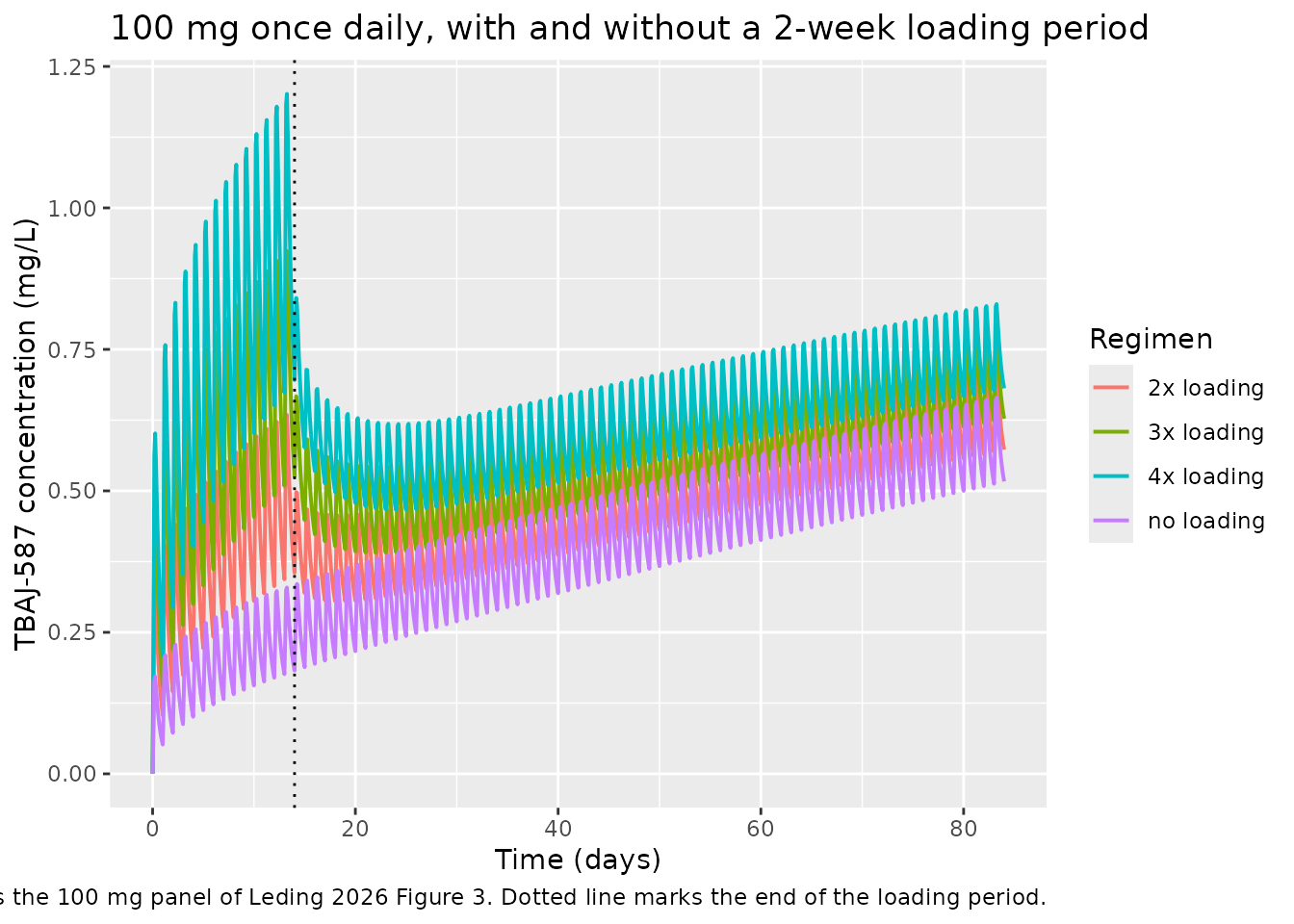
none <- cavg_tab[cavg_tab$ratio == 1, ]
load_only <- cavg_tab[cavg_tab$ratio > 1, ]

# 1. Loading doses raise early exposure (Results 3.3, "initially higher
#    concentrations"). Deterministic and large.
stopifnot(all(load_only$d14 / none$d14 > 1.5))

# 2. Steady state is NOT reached at 12 weeks: Cavg is still climbing between
#    week 8 and week 12 under every regimen.
stopifnot(all(cavg_tab$d84 / cavg_tab$d56 > 1.05))

# 3. The loading-vs-none gap narrows sharply once maintenance dosing starts.
#    This is the reproducible part of the paper's "similar at 4 weeks" claim;
#    see Assumptions and deviations for the part that is not.
gap_d14 <- load_only$d14 / none$d14 - 1
gap_d28 <- load_only$d28 / none$d28 - 1
stopifnot(all(gap_d28 < 0.5 * gap_d14))

cavg_tab |>
  dplyr::select(-ratio) |>
  dplyr::rename("Regimen" = regimen, "Day 14" = d14, "Day 28" = d28,
                "Day 56" = d56, "Day 84" = d84) |>
  knitr::kable(digits = 4, caption = paste(
    "Cavg (mg/L) of TBAJ-587 at 100 mg once daily maintenance, fed, by",
    "loading-dose ratio. Cavg = AUC0-24h / 24 (Leding 2026 Equation 5)."
))| Regimen | Day 14 | Day 28 | Day 56 | Day 84 |
|---|---|---|---|---|
| no loading | 0.2495 | 0.3266 | 0.4627 | 0.5847 |
| 2x loading | 0.4836 | 0.3997 | 0.5254 | 0.6410 |
| 3x loading | 0.7102 | 0.4709 | 0.5864 | 0.6958 |
| 4x loading | 0.9314 | 0.5408 | 0.6463 | 0.7495 |
Between-subject variability
The simulations above are typical-value replications of the paper’s own typical-value tables. This section exercises the IIV structure: 12 etas, of which 7 are fixed from the parent sub-model and 5 were estimated for the metabolites.
# set.seed() seeds R's RNG, NOT rxode2's -- and rxode2's streams are
# partitioned per solver thread, so this cohort differs between a 16-thread
# workstation and a 2-core CI runner. No assertion below depends on the
# particular draw.
set.seed(20260912)
n_per_arm <- 100L      # well under the 200/arm cap

vpc_arms <- c(50, 200, 800)
obs_grid <- c(seq(0, 24, by = 1), seq(30, 312, by = 6),
              seq(360, 126 * 24, by = 48))

events_vpc <- lapply(seq_along(vpc_arms), function(i) {
  D <- vpc_arms[i]
  base <- make_events(D, 0, obs_grid, fed = 0)
  base <- base[rep(seq_len(nrow(base)), times = n_per_arm), ]
  base$id <- rep((i - 1L) * n_per_arm + seq_len(n_per_arm),
                 each = nrow(base) / n_per_arm)
  base$treatment <- paste(D, "mg")
  base
}) |>
  dplyr::bind_rows()

# Disjoint ids across arms are mandatory: duplicates silently merge into one
# subject receiving the summed dose.
stopifnot(!anyDuplicated(unique(events_vpc[, c("id", "time", "evid")])))
stopifnot(dplyr::n_distinct(events_vpc$id) == n_per_arm * length(vpc_arms))

sim_vpc <- rxode2::rxSolve(readModelDb("Leding_2026_tbaj587"),
                           events = events_vpc, keep = "treatment") |>
  as.data.frame() |>
  dplyr::filter(!is.na(Cc))
#> ℹ parameter labels from comments will be replaced by 'label()'
sim_vpc |>
  dplyr::filter(time > 0, time <= 312) |>
  dplyr::group_by(treatment, time) |>
  dplyr::summarise(Q05 = quantile(Cc, 0.05), Q50 = quantile(Cc, 0.50),
                   Q95 = quantile(Cc, 0.95), .groups = "drop") |>
  ggplot(aes(time, Q50)) +
  geom_ribbon(aes(ymin = Q05, ymax = Q95), alpha = 0.25) +
  geom_line(linewidth = 0.7) +
  facet_wrap(~treatment) +
  scale_y_log10() +
  labs(x = "Time after a single dose (h)", y = "TBAJ-587 (mg/L)",
       title = "Simulated single-dose profiles with between-subject variability",
       caption = paste("Median and 5th-95th percentiles,", n_per_arm,
                       "subjects per arm. Comparable to the prediction-corrected",
                       "VPC in Leding 2026 Figure S1."))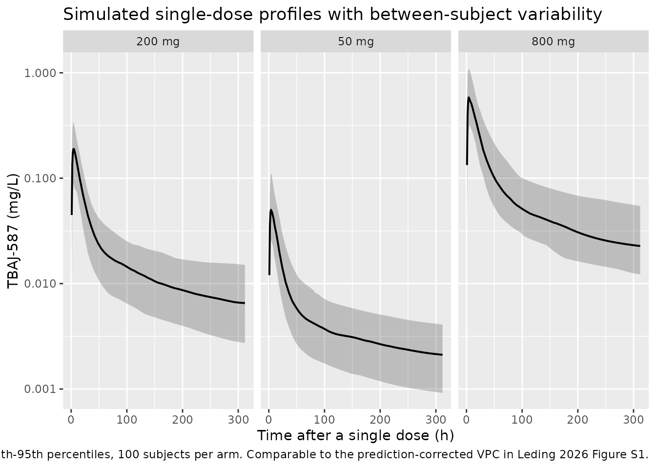
# The cohort median should track the typical-value prediction closely, and the
# IIV magnitude should land near the published CV%. Both are asserted as
# magnitudes with headroom, never as a sign, an equality, or a bound taken
# from one run.
cv_obs <- sim_vpc |>
  dplyr::filter(treatment == "200 mg", time == 312) |>
  dplyr::summarise(cv = stats::sd(Cc) / mean(Cc)) |>
  dplyr::pull(cv)

# Table 1 puts IIV on parent CL at 42.2% and on Vc at 48.2%; a single
# concentration late in the profile aggregates several of these. A cohort of
# 100 estimates a CV this size to roughly +/- 10% relative, so bound the
# plausible band generously -- it still goes red if the omega block were
# dropped (CV -> 0) or inflated by an order of magnitude.
stopifnot(cv_obs > 0.10, cv_obs < 1.50)
sprintf("Observed CV of Cc at 312 h, 200 mg arm: %.1f%% (n = %d)",
        100 * cv_obs, n_per_arm)
#> [1] "Observed CV of Cc at 312 h, 200 mg arm: 60.5% (n = 100)"
Verification summary
| Claim | Source | Achieved | Status |
|---|---|---|---|
| Mass balance clAUCinf = doseF*Stirling, all 3 analytes | Structural gate | max |ratio - 1| = 3e-05 | Pass |
| Parent AUC0-24h at week 4, 6 dose levels | Table S2 | median |diff| 0.09%, max 0.21% | Pass |
| M3 AUC0-24h at week 4 (parent-molar-equivalent) | Table S2 | max |diff| 2.47%, resolved as a MW ratio | Pass |
| M2 AUC0-24h at week 4 (parent-molar-equivalent) | Table S2 | max |diff| 2.73%, resolved as a MW ratio | Pass |
| MW difference between TBAJ-587 and M3 is ‘only 2%’ | Discussion | recovered 2.3% from Table S2 | Pass |
| Approximately dose-proportional for the parent, less so for M2 and M3 | Results 3.2 | dose-normalised span: parent 0.20, M3 0.63, M2 0.79 | Pass |
| Abundance order TBAJ-587 > M3 > M2 | Results 3.1 | 15.07 > 1.73 > 0.75 h*mg/L | Pass |
| Terminal half-life 3.5 to 9.0 months over 25-800 mg | Results 3.2 | 8.63 months at 25 mg, 3.48 at 800 mg | Pass |
| Loading doses give initially higher concentrations | Results 3.3 | day-14 Cavg +94% to +273% vs no loading | Pass |
| Steady state not reached after 12 weeks of dosing | Results 3.3 | Cavg still rising: day84/day56 = 1.16 to 1.26 | Pass |
| At 4 weeks, exposure similar between loading and no loading | Results 3.3 | gap narrows from +94%..+273% (day 14) to +22%..+66% (day 28), not to ~0 | Deviation |
Assumptions and deviations
Structure from Code S1, values from Table 1. The supplement’s final control stream carries the metabolite
$THETA/$OMEGArecords at their initial values, not their final ones (CLM320.121 vs 18.5;Q317.4191 vs 9.09;V6937.257 vs 1630). Every metabolite value in the model file therefore comes from Table 1, and every equation form from Code S1. The parent block isFIXin Code S1 at exactly its Table 1 values, so the two agree there;e_dose_kais taken from Code S1 (-0.000462) because Table 1 prints it rounded to two significant figures (-0.00046).The Stirling approximation is reproduced, not corrected. Code S1 normalises the Savic density with
LNFAC = LOG(2.5066)+(NN+0.5)*LOG(NN)-NNrather than the exactlgamma(NN+1). AtNN = 2.36that inflates the absorption input by 3.57%, so the model absorbs 1.0357 timesF * doserather than exactlyF * dose. Substituting the exact log-gamma would be “more correct” in isolation but would break consistency with the publishedCL, which was estimated against this expression; the same 3.57% bias is embedded in Table 1. The mass-balance gate targets the inflated value explicitly so the approximation is visible rather than hidden.Molar model, mass-unit validation table. The model is in nmol and nmol/L, matching Code S1. The paper reports no molecular weights, so none is invented. Parent exposures in mass units are molecular-weight-independent (verified numerically above), so the Table S2 parent comparison is exact. Metabolite exposures are reported in parent-molar-equivalent mass units and carry the factor
MW_metabolite / MW_parent, which this vignette recovers from Table S2 (M3 0.977, M2 0.978) rather than assuming. The recovered M3 ratio agrees with the paper’s stated 2% difference; the M2 ratio is unstated in the paper and is a prediction.fm_m2andfm_m3are anchored at 1, not summed to 1. Both relative fractions metabolised are fixed at 1 and each metabolite receives the parent’s whole elimination flux, so metabolite amounts are deliberately not mass-conserved against the parent and all metabolite clearances and volumes are apparent relative to an unidentifiable true fraction (Table 1 footnote a). This is faithful to Code S1, which retains the parent’s full-K20*A(2)term.fixed()marks only the by-fiat anchors.lfdepot,lfm_m2andlfm_m3are wrapped infixed(); they are the three parameters Table 1 reports as “1 FIX” with no RSE and no confidence interval. Every other value, includinglnn, carries an RSE and a SIR interval in Table 1 and so was estimated. Code S1 marks the whole parent blockFIXbecause the final model estimated the metabolite sub-models with the parent held at its own final estimates – an estimation-sequence device rather than a structurally fixed value, and not encoded asfixed()here.Deviation: “at 4 weeks, the exposure was similar between no loading doses and loading doses” (Results 3.3) is not reproduced quantitatively. At a 100 mg maintenance dose the day-28
Cavgremains +22%, +44% and +66% above the no-loading arm for the 2:1, 3:1 and 4:1 ratios. The direction of the claim is strongly reproduced – the gap collapses from +94%..+273% at day 14 to the day-28 values above – and with a terminal half-life of months, drug delivered during a 2-week loading period cannot have washed out by week 4, so a residual difference of this size is what the model’s own structure requires. The likely reading is that the claim is a visual one about Figure 3, where the curves have converged relative to their loading-period separation on an axis spanning the full 12 weeks. The claim is reported as a deviation and excluded from the render gate rather than having the gate widened until it passed.Not reproduced by design: the efficacy targets and safety references. Efficacy Targets 1 and 2 (Equations 3 and 4) are derived from bedaquiline and bedaquiline-M2 typical daily average concentrations taken from a separate published model (Leding 2026 reference 27) together with MIC-ratio potency corrections, and the safety references come from a 3-month dog toxicity study (reference 26). Neither the upstream bedaquiline model predictions nor the dog toxicity exposures are reproducible from this paper alone, so Figures 3-5’s horizontal target lines, and the conclusion that 100 mg once daily is the lowest regimen meeting both efficacy targets, are outside the scope of this validation. The TBAJ-587 exposure predictions that those lines are compared against are validated above.
Illustrative cohort. The between-subject-variability section simulates 100 subjects per arm at three of the six dose levels, fasted. The original observed data are not public, so it is a forward simulation from the packaged IIV rather than a true prediction-corrected VPC against Figure S1. Its assertions are written as magnitudes with headroom because rxode2’s RNG streams are partitioned per solver thread and a CI runner draws a different cohort.
BQL handling is not part of the packaged model. Leding 2026 omitted all parent below-quantification-limit records and all metabolite BQL records except the first and last in the decreasing and ascending curves, which were set to LLOQ/2 = 0.5 ng/mL (Results 3.1). That is an estimation-dataset decision with no simulation-time counterpart; simulated profiles here are not censored at the 1 ng/mL LLOQ.