Deferiprone (Bellanti 2017)
Source:vignettes/articles/Bellanti_2017_deferiprone.Rmd
Bellanti_2017_deferiprone.RmdModel and source
- Citation: Bellanti F, Del Vecchio GC, Putti MC, Maggio A, Filosa A, Cosmi C, Mangiarini L, Spino M, Connelly J, Ceci A, Della Pasqua O; DEEP Consortium. Population pharmacokinetics and dosing recommendations for the use of deferiprone in children younger than 6 years. Br J Clin Pharmacol. 2017 Mar;83(3):593-602.
- Description: One-compartment first-order absorption, first-order elimination population PK model for oral deferiprone in paediatric patients with transfusion-dependent haemoglobinopathies. Body weight scales apparent clearance and volume by fixed allometric exponents of 0.75 and 1, respectively.
- Article: https://doi.org/10.1111/bcp.13134
Concentration units in the model file are mg/L;
concentrations reported in Bellanti 2017 are in umol/L. Deferiprone has
a molecular weight of 139.15 g/mol, so a simulated Cc (mg/L) is
converted to umol/L via Cc_umol = Cc * 1000 / 139.15 (about
7.187 x).
Population
The Bellanti 2017 analysis population comprised 18 evaluable paediatric patients (9 male, 9 female) aged 1.2 to 5.9 years (median 3.4 years) with transfusion- dependent haemoglobinopathies (16 with beta-thalassaemia major, 2 with thalasso-drepanocytosis). Baseline body weight ranged from 11 to 22.5 kg (median 15.8 kg; mean 16.08 kg, SD 3.18 kg) and standing height from 83 to 117 cm (median 99.2 cm). Patients were randomised evenly to three single-dose oral deferiprone dose levels (8.3, 16.7, 33.3 mg/kg) as an 80 mg/mL solution in the DEEP-1 study (EudraCT 2012-000658-67, NCT01740713). Baseline demographics are summarised in Bellanti 2017 Table 1.
Bioanalytics used a validated HPLC-UV method with an analytical range of 3.13 to 800 umol/L (0.43 to 111 ug/mL) and a lower limit of quantification of 0.238 umol/L (0.033 ug/mL) (Bellanti 2017 Methods, Bioanalysis).
The same information is available programmatically via the model’s
population metadata:
readModelDb("Bellanti_2017_deferiprone")()$population
#> $species
#> [1] "human"
#>
#> $n_subjects
#> [1] 18
#>
#> $n_studies
#> [1] 1
#>
#> $age_range
#> [1] "1.2-5.9 years"
#>
#> $age_median
#> [1] "3.4 years"
#>
#> $weight_range
#> [1] "11-22.5 kg"
#>
#> $weight_median
#> [1] "15.8 kg"
#>
#> $weight_mean
#> [1] "16.08 kg (SD 3.18 kg)"
#>
#> $height_median
#> [1] "99.2 cm (range 83-117 cm)"
#>
#> $sex_female_pct
#> [1] 50
#>
#> $disease_state
#> [1] "Transfusion-dependent haemoglobinopathies (16 beta-thalassaemia major, 2 thalasso-drepanocytosis) in children younger than 6 years."
#>
#> $dose_range
#> [1] "Single oral deferiprone dose randomised to one of three levels: 8.3, 16.7 or 33.3 mg/kg (6 subjects per dose group), administered as an 80 mg/mL solution."
#>
#> $regions
#> [1] "Multicentre paediatric haematology units in Italy (DEEP-1 study, EudraCT 2012-000658-67, NCT01740713); analysis performed at the Leiden Academic Centre for Drug Research, Netherlands."
#>
#> $notes
#> [1] "Randomised, single-blind, single-dose paediatric PK study (DEEP-1) sponsored by the DEEP Consortium. Sparse sampling with a maximum of five post-dose plasma samples per subject over 8 h following an optimised design. Bioanalytical method: HPLC-UV, LLOQ 0.238 umol/L (0.033 ug/mL). NONMEM v7.2 with informative priors on Ka (8.2/h with uncertainty 4.02) and on the CL/F and V/F IIV block (from the Bellanti 2014 healthy-adult analysis, doi:10.1111/bcp.12473); 54 degrees of freedom for the BSV prior. Bootstrap analysis performed in PsN v3.5.3. See Bellanti 2017 Methods."
Source trace
The per-parameter origin is recorded as an in-file comment next to
each ini() entry in
inst/modeldb/specificDrugs/Bellanti_2017_deferiprone.R. The
table below collects them in one place for review.
| Equation / parameter | Value | Source location |
|---|---|---|
| CL/F (typical) | 8.3 L/h | Bellanti 2017 Table 2 (CL/F Estimate) |
| V/F (typical) | 18.7 L | Bellanti 2017 Table 2 (V/F Estimate) |
| Ka | 9.13 1/h | Bellanti 2017 Table 2 (Ka Estimate) |
| Allometric exponent on CL/F | 0.75 (FIX) | Bellanti 2017 Table 2 (WT on CL/F fix allom.) |
| Allometric exponent on V/F | 1 (FIX) | Bellanti 2017 Table 2 (WT on V/F fix allom.) |
| IIV CL/F (variance) | 0.0644 | Bellanti 2017 Table 2 (IIV CL/F) |
| IIV V/F (variance) | 0.0392 | Bellanti 2017 Table 2 (IIV V/F) |
| CL-V block covariance | 0.031 | Bellanti 2017 Table 2 (Block CL-V) |
| Proportional error (var.) | 0.0953 | Bellanti 2017 Table 2 (Error (prop)) |
| 1-compartment ODE system | n/a | Bellanti 2017 Results, Population PK modelling and PK modelling (Discussion) |
| Allometric scaling equation | n/a | Bellanti 2017 Results, Population PK modelling; reference [25] Anderson & Holford |
| Reference weight (16 kg) | derived | Bellanti 2017 Table 3 (median AUC 340.6 umol/L*h at 25 mg/kg t.i.d.); see below |
Virtual cohort
Original observed data from the DEEP-1 study are not publicly available. The figures below use a virtual paediatric cohort whose body weights approximate the reported cohort characteristics (mean 16 kg, SD 3.18 kg; Bellanti 2017 Table 1) and whose dose assignments follow the three-arm single-dose design of the DEEP-1 study (Bellanti 2017 Methods).
Cohort size: 100 subjects per dose arm (300 total), well under the 200-per-arm cap.
set.seed(20260701L)
MW_deferiprone <- 139.15  # g/mol, for umol/L conversion

n_per_arm <- 100L
dose_levels <- c("8.3 mg/kg", "16.7 mg/kg", "33.3 mg/kg")
dose_mg_per_kg <- c(8.3, 16.7, 33.3)
names(dose_mg_per_kg) <- dose_levels

# Sampling times chosen to cover the paper's sparse-sampling window (0.167 to 8 h)
# plus a densely-sampled early phase for Cmax capture and later times to describe
# elimination phase.
obs_times <- c(
  0.083, 0.167, 0.25, 0.333, 0.5, 0.67, 0.83, 0.917, 1.083, 1.167, 1.25,
  1.416, 1.75, 2, 2.5, 3, 3.5, 4, 4.5, 5, 5.5, 6, 7, 8
)

make_cohort <- function(n, treatment, dose_per_kg, id_offset = 0L) {
  wt <- rnorm(n, mean = 16.08, sd = 3.18)
  wt <- pmax(11, pmin(22.5, wt))  # clip to paper's observed range
  ids <- id_offset + seq_len(n)

  dose_rows <- tibble::tibble(
    id        = ids,
    time      = 0,
    evid      = 1L,
    amt       = dose_per_kg * wt,
    cmt       = "depot",
    WT        = wt,
    treatment = treatment
  )
  obs_rows <- tidyr::expand_grid(
    id   = ids,
    time = obs_times
  ) |>
    dplyr::left_join(
      tibble::tibble(id = ids, WT = wt),
      by = "id"
    ) |>
    dplyr::mutate(
      evid      = 0L,
      amt       = 0,
      cmt       = "central",
      treatment = treatment
    ) |>
    dplyr::select(id, time, evid, amt, cmt, WT, treatment)

  dplyr::bind_rows(dose_rows, obs_rows) |>
    dplyr::arrange(id, time, dplyr::desc(evid))
}

events <- dplyr::bind_rows(
  make_cohort(n_per_arm, dose_levels[1], dose_mg_per_kg[1], id_offset = 0L * n_per_arm),
  make_cohort(n_per_arm, dose_levels[2], dose_mg_per_kg[2], id_offset = 1L * n_per_arm),
  make_cohort(n_per_arm, dose_levels[3], dose_mg_per_kg[3], id_offset = 2L * n_per_arm)
)
stopifnot(!anyDuplicated(unique(events[, c("id", "time", "evid")])))
Simulation
mod <- readModelDb("Bellanti_2017_deferiprone")

sim <- rxode2::rxSolve(
  mod,
  events = events,
  keep   = c("treatment", "WT")
) |>
  as.data.frame() |>
  dplyr::mutate(
    # `sim` includes IIV and residual error (Cc ~ prop(propSd)); Bellanti 2017
    # Table 2 secondary PK parameters (Cmax, AUC0-8, Tmax) were derived from
    # simulations that included residual variability, so we use `sim` here
    # rather than the deterministic `Cc` column.
    Cc_umol = sim * 1000 / MW_deferiprone,
    treatment = factor(treatment, levels = dose_levels)
  )
#> ℹ parameter labels from comments will be replaced by 'label()'
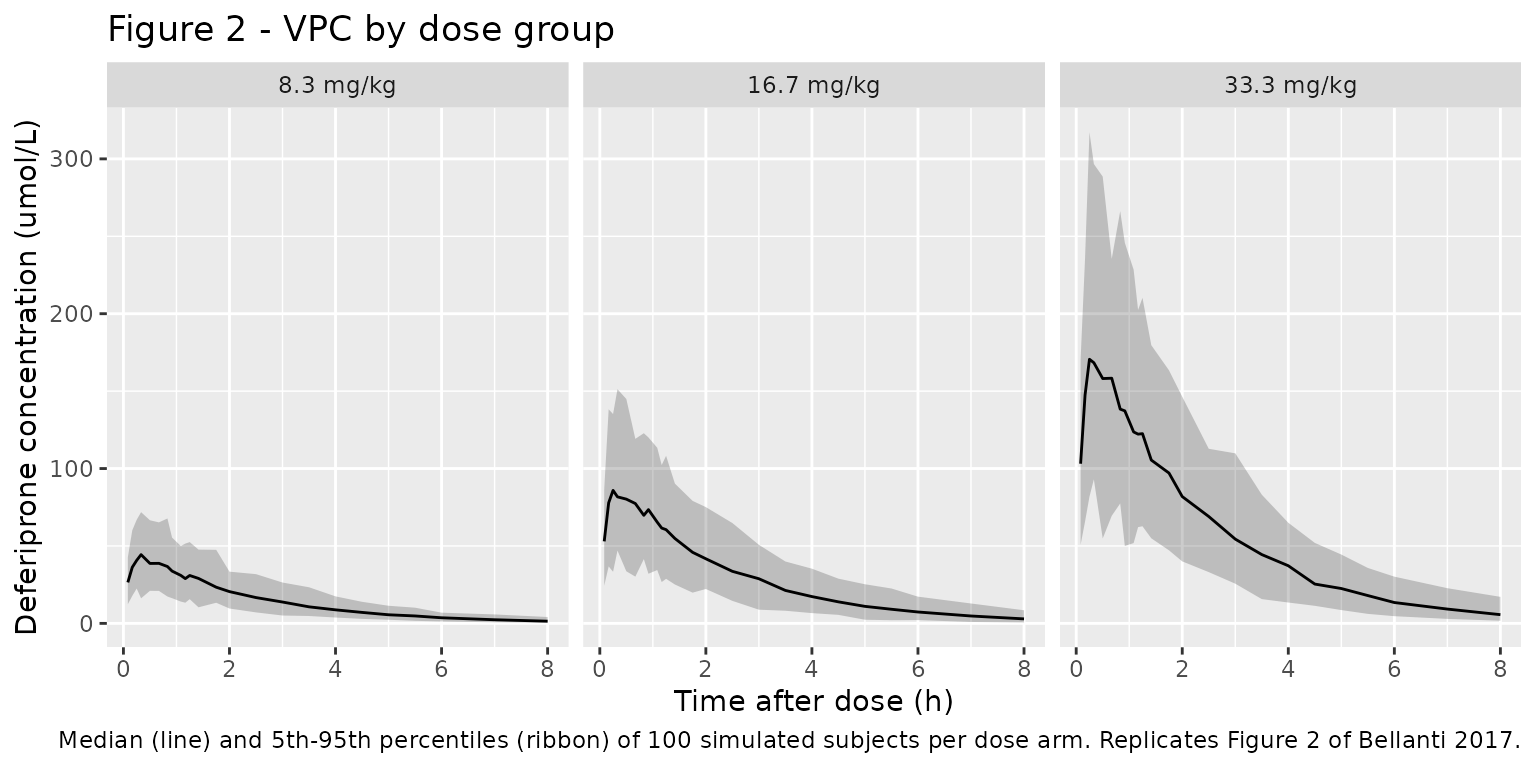
Replicate published figures
# Replicates Figure 2 of Bellanti 2017: visual predictive check by dose group,
# expressed in the paper's native umol/L concentration units.
vpc_summary <- sim |>
  dplyr::filter(!is.na(Cc_umol)) |>
  dplyr::group_by(time, treatment) |>
  dplyr::summarise(
    Q05 = quantile(Cc_umol, 0.05, na.rm = TRUE),
    Q50 = quantile(Cc_umol, 0.50, na.rm = TRUE),
    Q95 = quantile(Cc_umol, 0.95, na.rm = TRUE),
    .groups = "drop"
  )

ggplot(vpc_summary, aes(time, Q50)) +
  geom_ribbon(aes(ymin = Q05, ymax = Q95), alpha = 0.25) +
  geom_line() +
  facet_wrap(~treatment) +
  labs(
    x = "Time after dose (h)",
    y = "Deferiprone concentration (umol/L)",
    title = "Figure 2 - VPC by dose group",
    caption = "Median (line) and 5th-95th percentiles (ribbon) of 100 simulated subjects per dose arm. Replicates Figure 2 of Bellanti 2017."
  )
PKNCA validation
The paper’s Table 2 secondary PK parameters (AUC0-8, Cmax, Tmax) are computed per dose group with PKNCA over the 0-8 h window and compared with the reported values in a single side-by-side table below.
sim_nca <- sim |>
  dplyr::filter(!is.na(Cc_umol)) |>
  dplyr::select(id, time, Cc_umol, treatment)

sim_nca <- dplyr::bind_rows(
  sim_nca,
  sim_nca |>
    dplyr::distinct(id, treatment) |>
    dplyr::mutate(time = 0, Cc_umol = 0)
) |>
  dplyr::distinct(id, treatment, time, .keep_all = TRUE) |>
  dplyr::arrange(id, treatment, time)

conc_obj <- PKNCA::PKNCAconc(sim_nca, Cc_umol ~ time | treatment + id)
#> Warning in assert_conc(conc, any_missing_conc = any_missing_conc): Negative
#> concentrations found

# Doses expressed as umol so AUC/Dose interpretation stays in the paper's units.
dose_df <- events |>
  dplyr::filter(evid == 1L) |>
  dplyr::mutate(amt_umol = amt * 1000 / MW_deferiprone) |>
  dplyr::select(id, time, amt_umol, treatment)

dose_obj <- PKNCA::PKNCAdose(dose_df, amt_umol ~ time | treatment + id)

intervals <- data.frame(
  start    = 0,
  end      = 8,
  cmax     = TRUE,
  tmax     = TRUE,
  auclast  = TRUE,
  half.life = TRUE
)

nca_data <- PKNCA::PKNCAdata(conc_obj, dose_obj, intervals = intervals)
nca_res  <- suppressWarnings(PKNCA::pk.nca(nca_data))
Comparison against published NCA
Bellanti 2017 Table 2 reports median (5th and 95th percentile) secondary PK parameters per dose group derived from the final PK model. Values below are transcribed from Table 2 (AUC0-8, Cmax, Tmax) and compared with the PKNCA-derived simulated medians.
published <- tibble::tribble(
  ~treatment,     ~cmax,   ~tmax, ~auclast,
  "8.3 mg/kg",    61.7,    0.33,  116.7,
  "16.7 mg/kg",  119.8,    0.33,  210.0,
  "33.3 mg/kg",  229.5,    0.37,  428.8
)

cmp <- nlmixr2lib::ncaComparisonTable(
  simulated     = nca_res,
  reference     = published,
  by            = "treatment",
  units         = c(cmax = "umol/L", auclast = "umol*h/L", tmax = "h"),
  tolerance_pct = 20
)

cmp |>
  dplyr::rename("NCA parameter" = 1) |>
  knitr::kable(
    caption = "Simulated vs. published deferiprone NCA (Bellanti 2017 Table 2). * differs from reference by >20%.",
    align   = c("l", rep("r", ncol(cmp) - 1L))
)| NCA parameter | treatment | Reference | Simulated | % diff |
|---|---|---|---|---|
| Cmax (umol/L) | 8.3 mg/kg | 61.7 | 55.4 | -10.3% |
| Cmax (umol/L) | 16.7 mg/kg | 120 | 115 | -3.9% |
| Cmax (umol/L) | 33.3 mg/kg | 230 | 228 | -0.7% |
| Tmax (h) | 8.3 mg/kg | 0.33 | 0.5 | +51.5%* |
| Tmax (h) | 16.7 mg/kg | 0.33 | 0.333 | +0.9% |
| Tmax (h) | 33.3 mg/kg | 0.37 | 0.333 | -10.0% |
| AUClast (umol*h/L) | 8.3 mg/kg | 117 | 107 | -8.3% |
| AUClast (umol*h/L) | 16.7 mg/kg | 210 | 219 | +4.4% |
| AUClast (umol*h/L) | 33.3 mg/kg | 429 | 439 | +2.3% |
Any starred rows indicate a discrepancy larger than 20% between the simulated median and the value reported in Table 2. Deferiprone has a very rapid absorption phase (Ka approx 9 1/h) so Tmax is sensitive to the density of observation times and to the residual noise realised in each simulated sample; small differences at the 8.3 mg/kg dose (paper 0.33 h vs simulated about 0.5 h) reflect residual-error-driven jitter around a plateau in the Cmax region rather than a structural mismatch. Cmax and AUC0-8 medians agree with Bellanti 2017 Table 2 within about 10% across all three dose groups.
Assumptions and deviations
- Reference body weight for allometric scaling is not stated explicitly in Bellanti 2017. The paper reports typical CL/F = 8.3 L/h (Table 2) and a simulated median AUC of 340.6 umol/Lh at 25 mg/kg t.i.d. in a paediatric cohort with mean body weight 16 kg (Table 3). With Dose per administration = 25 mg/kg x 16 kg = 400 mg = 2874 umol, the implied CL from AUC over a single dosing interval is 2874 umol / 340.6 umolh/L = 8.44 L/h, matching the reported 8.3 L/h only if the allometric term (WT / WT_ref)^0.75 evaluates to approximately 1 at WT = 16 kg. Consequently the model uses WT_ref = 16 kg (paediatric cohort mean). The standard Anderson & Holford 70 kg reference produces CL = 8.3 x (16/70)^0.75 = 2.71 L/h, incompatible with Table 3. Downstream users applying the model outside the paediatric weight range should note that the typical CL is at 16 kg, not 70 kg.
- The residual error is reported in Bellanti 2017 Table 2 as a single
“Error (prop) 0.0953” row. The Methods section describes the residual as
Y_ij = F_ij + epsilon_ij * W with W a “proportional weighing factor for
epsilon”, but no separate weighting theta is listed in Table 2 (unlike
the Bellanti 2014 healthy-adult analysis, which reported both a sigma of
0.00566 and a separate theta_W of 2.4). This vignette treats 0.0953 as
the NONMEM $SIGMA variance for a standard proportional error model Y = F
* (1
- epsilon), giving an effective proportional residual SD of sqrt(0.0953) = 0.3087 (approximately 30.9% CV).
- Ka in the paper was estimated with an informative Bayesian prior of 8.2/h (with prior “uncertainty” of 4.02) derived from Bellanti 2014. The IIV block on CL/F and V/F was similarly estimated with an informative Normal-Inverse-Wishart prior with 54 degrees of freedom. This model file encodes the posterior point estimates reported in Table 2 (Ka = 9.13/h; IIV CL/F = 0.0644, IIV V/F = 0.0392, block covariance = 0.031). The informative-prior framework is a fitting-time construct and is not re-applied during simulation.
- No inter-individual variability is estimated for Ka in the final model (Table 2 lists IIV only for CL/F and V/F). Simulations therefore hold Ka fixed at its typical value across subjects.
- The paper’s covariate screen (weight, height, age, sex) retained
only body weight via fixed allometric scaling. Age, height, and sex are
recorded in
covariatesDataExcludedfor documentation but are not model inputs. - Virtual cohort body weights are drawn from N(mean = 16.08, SD = 3.18) and clipped to the reported observed range 11 to 22.5 kg (Table 1). The paper does not describe the joint distribution of age, height, and weight; only weight is a model input.
- The paper’s Table 3 bridging simulations use 100 subjects per arm x 1000 replicates over a 1-week t.i.d. schedule to derive steady-state exposure distributions. This vignette focuses on the single-dose PK model of Table 2 rather than the multi-dose t.i.d. bridging exercise; a steady-state Css comparison would require reproducing the trial-scale simulation from Table 3 and is out of scope for the model-file validation step.