Antibacterial efficacy: 5 antibiotics vs S. pyogenes (Nielsen 2011) • nlmixr2lib

Model and source

Citation: Nielsen EI, Cars O, Friberg LE. (2011). Predicting in vitro antibacterial efficacy across experimental designs with a semimechanistic pharmacokinetic-pharmacodynamic model. Antimicrobial Agents and Chemotherapy 55(4):1571-1579. doi:10.1128/AAC.01286-10. Model structure originally developed in Nielsen EI, Viberg A, Lowdin E, Cars O, Karlsson MO, Sandstrom M. (2007). Semimechanistic pharmacokinetic/pharmacodynamic model for assessment of activity of antibacterial agents from time-kill curve experiments. Antimicrob Agents Chemother 51(1):128-136 (reference 31 in Nielsen 2011); the 2011 paper extends the same structure to dynamic concentration-time profiles and reports re-estimated parameters.
Article: https://doi.org/10.1128/AAC.01286-10

This is not a population PK model. It is a semimechanistic in-vitro PKPD model of bacterial growth and killing fit with NONMEM (Laplacian, version VI) to natural-log viable count measurements from time-kill curve experiments of Streptococcus pyogenes exposed to five antibiotics of different classes: benzylpenicillin (PEN), cefuroxime (CXM), erythromycin (ERY), moxifloxacin (MXF), and vancomycin (VAN). The five drugs share a common bacterial-growth structure (the proliferating-sensitive / non-growing-resting two-stage life-cycle of Nielsen 2007, reference 31 of the 2011 paper) and differ only in their drug-specific PK (degradation kdeg, effect-compartment delay ke0) and PD (Emax, EC50, Hill exponent gamma) parameter values. Because the paper fit all five drugs jointly in one NONMEM estimation but each individual experiment exposed one drug at a time, the library packages each drug as a standalone file (Nielsen_2011_<drug>.R), and this vignette walks through the shared structure and reproduces the published kill / regrowth behaviour for each.

PKNCA / NCA is not an appropriate validation: there is no absorption-distribution-elimination profile of a drug to integrate (the in vitro drug concentration is dosed directly into the broth and declines exponentially per the kinetic-system flow rate plus drug degradation). The checks below are the mechanistic equivalents (growth-control hits the carrying-capacity, sub-MIC trajectories stabilize near the inoculum, supra-MIC trajectories kill rapidly, and dynamic regimens reproduce the qualitative kill / regrowth pattern of paper Figure 3).

Population (biological context)

Streptococcus pyogenes group A strain M12 NCTC P1800 (National Culture Type Collection) grown in Todd-Hewitt broth at 35 C, with a target starting inoculum of 10^6 CFU/mL from a 6-h logarithmic-growth-phase culture. Static experiments used 10-mL test tubes (4 mL broth); dynamic experiments used a 110-mL open-bottom spinner-flask in vitro kinetic system with pump-driven medium dilution producing first-order antibiotic elimination at a flow rate chosen to mimic each drug’s reported human plasma half-life (Table 1 of the source). Most experiments ran 24 h (some 48 h). The limit of detection was 10 CFU/mL.

The model was fit simultaneously to all five drugs using NONMEM’s mixture module to allow two subpopulations of experiments differing in the starting-fraction of resting bacteria (Methods, “Semimechanistic PKPD model”).

The same information is available programmatically via readModelDb("Nielsen_2011_benzylpenicillin")$population (and analogous calls for the other four drugs).

Source trace

Per-parameter origins are recorded as in-file comments next to each ini() entry in inst/modeldb/specificDrugs/Nielsen_2011_<drug>.R. All values come from the Nielsen 2011 paper’s “Static and dynamic” column of Table 3 (the combined-data joint fit) plus Table 1 (simulated human half-lives) and the Methods section (drug degradation rates, starting inoculum).

Equation / parameter	Value	Source location
`kgrowth` (bacterial multiplication)	1.46 /h	Table 3 column “Static and dynamic”
`kdeath` (natural death)	0.187 /h	Table 3 column “Static and dynamic”
`Bmax` (carrying capacity)	5.00 x 10^8 CFU/mL	Table 3 column “Static and dynamic”
`fpers` (resting fraction at t=0, subpop 2)	0.0652	Table 3 column “Static and dynamic”
`fMix1` (proportion of subpop 1)	0.880	Table 3 column “Static and dynamic”
`Emax` per drug	2.70 (PEN), 2.72 (CXM), 2.46 (ERY), 3.40 (MXF), 1.52 (VAN) /h	Table 3 column “Static and dynamic”
`EC50` per drug	0.00531, 0.00787, 0.0336, 0.0750, 0.304 mg/L	Table 3 column “Static and dynamic”
gamma (Hill exponent) per drug	1.06, 1.35, 0.652, 1.42, 4.99	Table 3 column “Static and dynamic”
`ke0` per drug	100 FIX (PEN/CXM/VAN), 1.02 (ERY), 0.627 (MXF) /h	Table 3 column “Static and dynamic”
`kdeg` per drug (in-broth degradation)	0.020 (PEN), 0.026 (CXM), 0 (ERY/MXF/VAN) /h	Methods “Semimechanistic PKPD model”
Simulated human half-life per drug	1.0 (PEN), 1.7 (CXM), 1.7 (ERY), 12.7 (MXF), 5.1 (VAN) h	Table 1
Starting inoculum	10^6 CFU/mL	Methods “Time-kill curve experiments”
Residual error (additive on natural log)	eps = 1.40 (common) + epsrepl = 0.468 (replicate)	Table 3 column “Static and dynamic”
Eq 1: `dC/dt = -keC - kdegC`	n/a	Page 1573
Eq 2: `dCe/dt = ke0C - ke0Ce`	n/a	Page 1573
Eq 3: `dS/dt = kgrowthS - (kdeath + drug)S - kSR*S`	n/a	Page 1573
Eq 4: `dR/dt = kSRS - kdeathR`	n/a	Page 1573
Eq 5: `kSR = (kgrowth - kdeath)/Bmax * (S + R)`	n/a	Page 1573
Eq 6: `drug = Emax * Ce^gamma / (Ce^gamma + EC50^gamma)`	n/a	Page 1573

Units (dimensional analysis)

Symbol	Meaning	Units
`central` (state)	drug concentration in broth	mg/L
`effect` (state)	effect-compartment concentration	mg/L
`bact_sensitive`, `bact_resting` (states)	bacterial counts	CFU/mL
`kgrowth`, `kdeath`, `ke`, `ke0`, `kdeg`, `kSR`, `Emax`, `drug_kill`	rate constants	1/h
`EC50`	half-effect concentration	mg/L
gamma (`hill`), `fpers`, `fMix1`, `f_resting_t0`	dimensionless	–
`Bmax`, `cfu0`	bacterial reference counts	CFU/mL

Each growth / kill ODE term has (1/h) * (CFU/mL) = (CFU/mL)/h, matching d/dt(state); each drug ODE term has (1/h) * (mg/L) = (mg/L)/h. The sigmoidal-Emax killing term Emax * Ce^gamma / (EC50^gamma + Ce^gamma) has units (1/h) * (mg/L)^gamma / (mg/L)^gamma = 1/h. The kSR reparameterisation (kgrowth - kdeath) / Bmax * (S+R) carries (1/h) / (CFU/mL) * (CFU/mL) = 1/h.

Drug overview

drugs <- c("benzylpenicillin", "cefuroxime", "erythromycin", "moxifloxacin", "vancomycin")
abbrev <- c("PEN", "CXM", "ERY", "MXF", "VAN")
mic    <- c(0.012, 0.0313, 0.125, 0.125, 0.25)  # mg/L (Table 1)
thalf  <- c(1.0, 1.7, 1.7, 12.7, 5.1)          # h (Table 1)
emax   <- c(2.70, 2.72, 2.46, 3.40, 1.52)      # /h (Table 3 "Static and dynamic")
ec50   <- c(0.00531, 0.00787, 0.0336, 0.0750, 0.304)
gamma  <- c(1.06, 1.35, 0.652, 1.42, 4.99)
ke0    <- c(100, 100, 1.02, 0.627, 100)
kdeg   <- c(0.020, 0.026, 0, 0, 0)
knitr::kable(data.frame(
  drug = drugs, abbrev = abbrev, MIC_mgL = mic, t_half_h = thalf,
  Emax_h = emax, EC50_mgL = ec50, gamma = gamma, ke0_h = ke0, kdeg_h = kdeg
), digits = 4, caption = "Per-drug Table 1 (MIC, t1/2) and Table 3 'Static and dynamic' (PD) values.")

Per-drug Table 1 (MIC, t1/2) and Table 3 ‘Static and dynamic’ (PD) values.
drug	abbrev	MIC_mgL	t_half_h	Emax_h	EC50_mgL	gamma	ke0_h	kdeg_h
benzylpenicillin	PEN	0.0120	1.0	2.70	0.0053	1.060	100.000	0.020
cefuroxime	CXM	0.0313	1.7	2.72	0.0079	1.350	100.000	0.026
erythromycin	ERY	0.1250	1.7	2.46	0.0336	0.652	1.020	0.000
moxifloxacin	MXF	0.1250	12.7	3.40	0.0750	1.420	0.627	0.000
vancomycin	VAN	0.2500	5.1	1.52	0.3040	4.990	100.000	0.000

mods <- setNames(lapply(drugs, function(d) {
  rxode2::rxode(readModelDb(paste0("Nielsen_2011_", d)))
}), drugs)
mods[[1]]$state
#> [1] "central"        "effect"         "bact_sensitive" "bact_resting"

Growth-control check (no drug)

With no antibiotic, the population grows from 10^6 toward the carrying-capacity Bmax = 5.00 x 10^8 CFU/mL through the joint operation of kgrowth and the density-dependent transfer kSR = (kgrowth-kdeath)/Bmax * (S+R). All five drug files share the bacterial-growth parameters, so any one of them suffices for this check. Paper Figure 2 reports that growth-control trajectories agreed between the static and dynamic systems and reached ~10^9 CFU/mL by ~10-12 h.

mod <- mods[["benzylpenicillin"]]
ev_gc <- rxode2::et(seq(0, 24, by = 0.5))
gc <- rxode2::rxSolve(mod, ev_gc, returnType = "data.frame", maxsteps = 1e5)
gc$btot <- exp(gc$Cc) - 1   # natural-log Cc -> CFU/mL

cat(sprintf("Inoculum  CFU(0)  = %.3e  (target 1.0e+06)\n", gc$btot[1]))
#> Inoculum  CFU(0)  = 1.000e+06  (target 1.0e+06)
cat(sprintf("At t=24h  CFU(24) = %.3e  (target Bmax = 5.0e+08)\n",
            tail(gc$btot, 1)))
#> At t=24h  CFU(24) = 5.360e+08  (target Bmax = 5.0e+08)

ggplot(gc, aes(time, btot)) +
  geom_line(linewidth = 1) +
  geom_hline(yintercept = 5e8, linetype = 2, colour = "grey50") +
  scale_y_log10() +
  labs(x = "Time (h)", y = "Bacterial count (CFU/mL)",
       title = "Growth control (no drug)",
       caption = "Dashed line: Bmax = 5.0e+08 CFU/mL (Table 3 Static and dynamic).")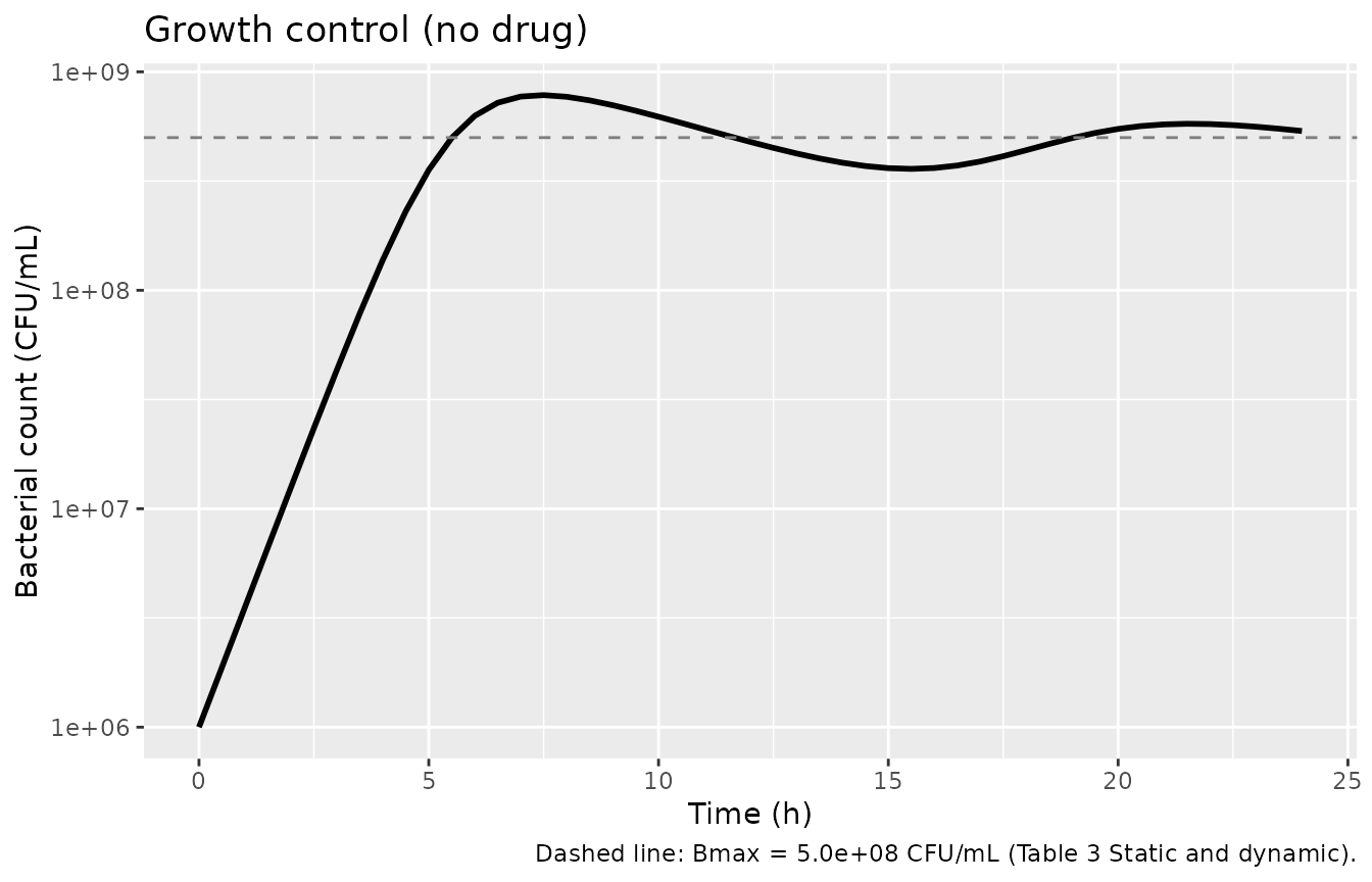

Static time-kill: reproduces Figure 5 behaviour

Paper Figure 5 shows static time-kill curves at concentrations spanning sub-MIC to ~64x MIC. We reproduce the qualitative kill / regrowth behaviour for each of the five drugs at 0.25, 1, 4, and 16 multiples of the MIC, with the in-vitro elimination rate ke set near zero (no flow). Drug degradation kdeg is retained at the published value for PEN and CXM (0.020 and 0.026 /h); ERY, MXF, VAN have kdeg = 0.

multiples <- c(0.25, 1, 4, 16)
times <- seq(0, 24, by = 0.5)

run_static <- function(drug, mult_mic) {
  mod <- mods[[drug]]
  amt <- mult_mic * mic[match(drug, drugs)]
  ev <- rxode2::et(amt = amt, cmt = "central", time = 0)
  ev <- rxode2::et(ev, times)
  sim <- rxode2::rxSolve(mod, ev,
                         params = c(lke = log(1e-9)),   # static -> ke ~ 0
                         returnType = "data.frame", maxsteps = 1e5)
  sim$drug <- drug
  sim$abbrev <- abbrev[match(drug, drugs)]
  sim$mult_mic <- mult_mic
  sim$btot <- exp(sim$Cc) - 1
  sim
}

static_sim <- bind_rows(lapply(drugs, function(d) {
  bind_rows(lapply(multiples, function(m) run_static(d, m)))
}))

ggplot(static_sim,
       aes(time, pmax(btot, 1), colour = factor(mult_mic))) +
  geom_line(linewidth = 0.7) +
  facet_wrap(~ abbrev, ncol = 5) +
  scale_y_log10(limits = c(1, 1e9)) +
  scale_colour_brewer("Initial concn (x MIC)", palette = "RdYlBu", direction = -1) +
  labs(x = "Time (h)", y = "Bacterial count (CFU/mL)",
       title = "Static time-kill curves",
       caption = paste("Reproduces Figure 5 of Nielsen 2011 (qualitative).",
                       "Sub-MIC: bacteria approach carrying capacity.",
                       "Supra-MIC: rapid kill to LOD with persister floor.")) +
  theme(legend.position = "bottom")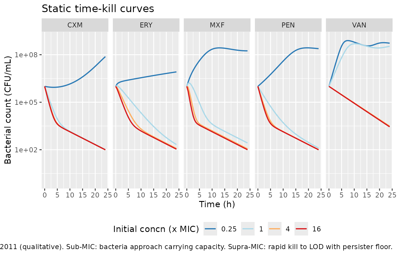

Dynamic time-kill: reproduces Figure 3 behaviour

Paper Figure 3 shows dynamic time-kill curves with starting concentrations of 2 and 16x MIC and simulated half-lives matching each drug’s human plasma half-life (Table 1). We reproduce the 16x MIC dynamic-human-t1/2 case for each drug. The default lke in each model file is set to log(ln(2)/t1/2_human) so no parameter override is needed; for the constant-concentration (“16:c”) case we override lke to ~0.

run_dynamic <- function(drug, mult_mic, kinetic_mode) {
  # kinetic_mode: "human" -> Table 1 simulated human t1/2 (default lke);
  #               "constant" -> lke ~ 0 (override).
  mod <- mods[[drug]]
  amt <- mult_mic * mic[match(drug, drugs)]
  ev <- rxode2::et(amt = amt, cmt = "central", time = 0)
  ev <- rxode2::et(ev, seq(0, 24, by = 0.5))
  if (kinetic_mode == "constant") {
    sim <- rxode2::rxSolve(mod, ev,
                           params = c(lke = log(1e-9)),
                           returnType = "data.frame", maxsteps = 1e5)
  } else {
    sim <- rxode2::rxSolve(mod, ev,
                           returnType = "data.frame", maxsteps = 1e5)
  }
  sim$drug <- drug
  sim$abbrev <- abbrev[match(drug, drugs)]
  sim$mode <- kinetic_mode
  sim$mult_mic <- mult_mic
  sim$btot <- exp(sim$Cc) - 1
  sim
}

dynamic_sim <- bind_rows(lapply(drugs, function(d) {
  bind_rows(
    run_dynamic(d, 16, "human"),
    run_dynamic(d, 16, "constant"),
    run_dynamic(d, 2,  "human")
  )
}))
dynamic_sim$panel <- with(dynamic_sim, paste0(mult_mic, ":", substr(mode, 1, 1)))

ggplot(dynamic_sim,
       aes(time, pmax(btot, 1), colour = panel)) +
  geom_line(linewidth = 0.7) +
  facet_wrap(~ abbrev, ncol = 5) +
  scale_y_log10(limits = c(1, 1e9)) +
  scale_colour_brewer("Regimen", palette = "Set1") +
  labs(x = "Time (h)", y = "Bacterial count (CFU/mL)",
       title = "Dynamic and constant-concentration time-kill",
       caption = paste("Reproduces Figure 3 of Nielsen 2011 (qualitative).",
                       "Regimen labels: 2:h = 2x MIC simulated human t1/2;",
                       "16:h = 16x MIC simulated human t1/2;",
                       "16:c = 16x MIC constant concentration (ke ~ 0).")) +
  theme(legend.position = "bottom")
#> Warning: Removed 4 rows containing missing values or values outside the scale range
#> (`geom_line()`).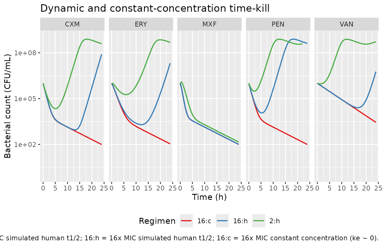

The structural prediction matches the paper’s qualitative narrative: PEN and CXM (short t1/2 of 1.0 and 1.7 h) regrow substantially over 24 h because the drug is rapidly cleared; MXF (12.7-h t1/2) and VAN (5.1-h t1/2) sustain killing because drug persists. Constant-concentration (“c”) gives the most sustained suppression in every drug.

Drug concentration check

The model’s drug ODE is dC/dt = -ke * C - kdeg * C. The effective decline rate is ke + kdeg so the realized half-life is shorter than the simulated t1/2 alone for PEN and CXM (which carry nonzero kdeg). Verify this against Table 1:

chk <- data.frame(
  drug = drugs,
  abbrev = abbrev,
  ke_default = log(2) / thalf,
  kdeg = kdeg,
  total_decline = log(2) / thalf + kdeg,
  effective_thalf = log(2) / (log(2) / thalf + kdeg)
)
knitr::kable(chk, digits = 3,
             caption = "Effective half-life = ln(2) / (ke + kdeg). PEN drops from 1.00 h to 0.97 h, CXM from 1.70 h to 1.64 h once degradation is added.")

Effective half-life = ln(2) / (ke + kdeg). PEN drops from 1.00 h to 0.97 h, CXM from 1.70 h to 1.64 h once degradation is added.
drug	abbrev	ke_default	kdeg	total_decline	effective_thalf
benzylpenicillin	PEN	0.693	0.020	0.713	0.972
cefuroxime	CXM	0.408	0.026	0.434	1.598
erythromycin	ERY	0.408	0.000	0.408	1.700
moxifloxacin	MXF	0.055	0.000	0.055	12.700
vancomycin	VAN	0.136	0.000	0.136	5.100

Assumptions and deviations

Mixture model collapsed to a typical-value initial condition. Nielsen 2011 used NONMEM’s mixture module to allow two subpopulations of experiments: subpopulation 1 (fMix1 = 0.880 of experiments) with no resting bacteria at t = 0, and subpopulation 2 (1 - fMix1 = 0.120 of experiments) with a resting fraction fpers = 0.0652 at t = 0. nlmixr2 / rxode2 does not support an analogous mixture-model construct for deterministic simulation, so each packaged model file uses the mixture-weighted mean fraction E[f_resting] = (1 - fMix1) * fpers = 0.00782 as a single typical-value starting condition. To simulate subpopulation 1 specifically, override fMix1 = 1 (or fpers = 0); to simulate subpopulation 2, override fMix1 = 0.
Residual error combined into a single additive SD. The source split the additive natural-log residual error into a common component (eps = 1.40) shared across an experiment’s replicate measurements and a replicate-specific component (epsrepl = 0.468). For a typical-use simulation drawing one observation per time point, the combined SD is sqrt(eps^2 + epsrepl^2) = sqrt(1.40^2 + 0.468^2) = 1.476. The packaged addSd carries this combined value.
Random effects (eta) are NOT included. The source NONMEM run estimated only the mixture-model variability in the resting fraction at t = 0 plus the additive residual error described above; it did not estimate eta-style between-experiment variability on the structural parameters. The packaged model is therefore intended for typical-value deterministic simulation (rxode2::rxSolve(mod, events)); there is no between-experiment IIV to draw from.
ke and kdeg are model parameters, not covariates. The in vitro kinetic-system elimination rate ke = ln(2) / simulated-half-life is fixed in each model file to its drug-specific simulated human t1/2 from Table 1 (the most commonly reported dynamic regimen). Users simulating a different half-life or a static experiment should override lke via rxode2::rxSolve(mod, events, params = c(lke = log(<new_ke>))); setting lke = log(1e-9) effectively zeroes out flow elimination for a static-concentration simulation. Per-drug kdeg (in-broth degradation) is fixed at the Methods-section value and is not user-controllable.
Sub-MIC behaviour at 0.25 x MIC. The model produces an apparent decline followed by slow recovery in sub-MIC simulations even when drug is below MIC, because the sigmoidal Emax killing function with EC50 near the MIC produces a non-zero drug_kill term at low concentrations. This is a property of the published equations (Eq 6), not a packaging deviation.
Vancomycin Discussion caveat. The paper Discussion notes that the model under-predicts the sustained suppression of bacterial growth observed for vancomycin at 2x MIC in dynamic experiments; this is a known source-paper limitation, not a translation error. Users simulating that specific regimen should expect a discrepancy with the paper’s measured time-kill curves at low concentrations.
No PKNCA / NCA validation. Standard PKNCA validation is not applicable to an in vitro PD-model output of bacterial count, so the endogenous-validation.md mechanistic-validation pattern is used instead (growth-control check, static / dynamic kill behaviour, dimensional analysis).