Olanzapine, rat striatum D2RO (Johnson 2011)
Source:vignettes/articles/Johnson_2011_olanzapine_rat.Rmd
Johnson_2011_olanzapine_rat.RmdModel and source
- Citation: Johnson M, Kozielska M, Pilla Reddy V, Vermeulen A, Li C, Grimwood S, de Greef R, Groothuis GMM, Danhof M, Proost JH. Mechanism-Based Pharmacokinetic-Pharmacodynamic Modeling of the Dopamine D2 Receptor Occupancy of Olanzapine in Rats. Pharm Res. 2011;28(10):2490-2504. doi:10.1007/s11095-011-0477-7.
- Description: hybrid physiology-based PK-PD model for olanzapine plasma and brain disposition coupled to a striatal D2 receptor binding state in rats; structural parameters per kg body weight.
Population
The Johnson 2011 dataset pooled 12 single-dose studies contributed by Janssen (Belgium), Merck Sharp and Dohme (The Netherlands), and Pfizer (USA) to the TI Pharma mechanism-based PK-PD platform: 283 adult Wistar or Sprague-Dawley rats receiving olanzapine 0.01-40 mg/kg by intraperitoneal (IP), subcutaneous (SC), or intravenous (IV) routes. D2 receptor occupancy was measured either in vivo with [3H]raclopride or ex vivo with [125I]sulpiride (Table I); the authors report no covariate effect on the plasma PK parameters and pool the two binding assays into a single PD model. All structural parameters in the file are body-weight normalised (per kg), reflecting how the source paper reports them.
The same information lives inside the model function
(population element of the
Johnson_2011_olanzapine_rat() definition in
inst/modeldb/specificDrugs/Johnson_2011_olanzapine_rat.R).
Source trace
The per-parameter origin is recorded as an in-file comment next to
each ini() entry in
inst/modeldb/specificDrugs/Johnson_2011_olanzapine_rat.R.
The table below collects them for review.
| Block | Symbol | Value | Source |
|---|---|---|---|
| Plasma PK (Table III) | V1 (Vc) | 4.22 L/kg | Table III, RSE 9% |
| Plasma PK | CL | 3.21 L/h/kg | Table III, RSE 9% |
| Plasma PK | V2 (Vp) | 2.23 L/kg | Table III, RSE 14% |
| Plasma PK | Q | 1.70 L/h/kg | Table III, RSE 30% |
| Plasma PK | FIP | 0.636 | Table III, RSE 12% |
| Plasma PK | FSC | 1 (fixed) | Results / Population Plasma PK; encoded as ROUTE_IP=0 collapsing to F=1 |
| Plasma PK | IAV-CL | 56% CV | Table III, RSE 19% (omega^2 = 0.3136 via paper’s omega^2 = (CV/100)^2 convention) |
| Plasma PK | IAV-F1 | 87% CV | Table III, RSE 18% (omega^2 = 0.7569; applied to FIP only via ROUTE_IP indicator) |
| Plasma PK | Proportional error | 0.141 | Table III, RSE 7% (log-additive; mapped to nlmixr2 prop()) |
| Brain physiology (fixed) | Vbv | 0.00024 L/kg | Methods, ref. 18 |
| Brain physiology (fixed) | Vbev | 0.00656 L/kg | Methods, ref. 18 |
| Brain physiology (fixed) | CLbv | 0.312 L/h/kg | Methods, ref. 18 (rat cerebral blood flow) |
| Binding (fixed) | fu_plasma | 0.23 | Methods, ref. 19 |
| Binding (fixed) | fu_brain | 0.034 | Methods, ref. 19 |
| Brain PK (Table V) | CLbev | 0.394 L/h/kg | Table V, RSE 15% |
| Receptor binding | Kd | 14.7 nM | Table V, RSE 8% |
| Receptor binding | koff | 2.62 1/h | Table V, RSE 24% |
| Receptor binding | kon (derived) | 0.178 nM^-1 h^-1 | koff / Kd (Methods) |
| Residual | Brain proportional | 0.479 | Table V, RSE 6% (matches Discussion “48% residual variability for brain”) |
| Residual | D2RO additive | 0.136 | Table V, RSE 5% |
| ODEs | central, peripheral1, brain_vascular, brain_extravascular, effect | n/a | Appendix 1 reduced model |
| Final-model rationale | Bmax dropped from full model | n/a | Results, Hybrid Physiology-Based PK-PD Model + Discussion |
Load the typical-value model
The published figures are typical-value (population-mean)
predictions, so we zero the between-animal variability for plotting and
put it back for the stochastic predictive check at the end. The encoding
f(central) <- exp(ROUTE_IP * (lfip + etalfip)) collapses
to F = 1 when ROUTE_IP = 0 (SC or IV) and to FIP with IIV when ROUTE_IP
= 1 (IP), so a single binary indicator covers all three routes used in
the source paper.
mod         <- readModelDb("Johnson_2011_olanzapine_rat")
mod_typical <- rxode2::zeroRe(mod)
Helpers
# Build a single-subject event table for one bolus dose of `amt` (mg/kg) into
# the central compartment with route-specific bioavailability. `route` is one
# of "IP", "SC", or "IV"; only IP uses the estimated FIP.
make_events <- function(amt_mgkg, route = c("SC", "IP", "IV"),
                        tmax = 24, dt = 0.05, id = 1L) {
  route <- match.arg(route)
  times <- seq(0, tmax, by = dt)
  route_ip <- as.integer(route == "IP")
  obs_Cc     <- data.frame(id = id, time = times, evid = 0, amt = 0,
                           rate = NA_real_, cmt = "Cc",
                           ROUTE_IP = route_ip)
  obs_Cbrain <- data.frame(id = id, time = times, evid = 0, amt = 0,
                           rate = NA_real_, cmt = "Cbrain",
                           ROUTE_IP = route_ip)
  obs_D2RO   <- data.frame(id = id, time = times, evid = 0, amt = 0,
                           rate = NA_real_, cmt = "D2RO",
                           ROUTE_IP = route_ip)
  dose <- data.frame(id = id, time = 0, evid = 1, amt = amt_mgkg,
                     rate = NA_real_, cmt = "central",
                     ROUTE_IP = route_ip)
  dplyr::bind_rows(dose, obs_Cc, obs_Cbrain, obs_D2RO)
}
Replicating Figure 3 – olanzapine 3 mg/kg SC
Figure 3 of Johnson 2011 plots observed olanzapine plasma and brain concentrations and striatal D2RO over time after a 3 mg/kg SC dose, overlaid with the typical-value model prediction. We reproduce the typical-value lines here; the open-circle observations are paper-specific animal data that were not released.
ev_3sc <- make_events(amt_mgkg = 3, route = "SC", tmax = 8, dt = 0.02)
sim_3sc <- as.data.frame(rxode2::rxSolve(mod_typical, ev_3sc))
#> ℹ omega/sigma items treated as zero: 'etalcl', 'etalfip'
sim_3sc_long <- sim_3sc |>
  dplyr::transmute(
    time,
    `Plasma (ng/mL)` = Cc     * 1000,
    `Brain  (ng/mL)` = Cbrain * 1000,
    `D2RO (fraction)` = D2RO
  ) |>
  tidyr::pivot_longer(-time, names_to = "panel", values_to = "value") |>
  dplyr::mutate(panel = factor(panel,
                               levels = c("Plasma (ng/mL)",
                                          "Brain  (ng/mL)",
                                          "D2RO (fraction)")))

ggplot(sim_3sc_long, aes(time, value)) +
  geom_line(linewidth = 0.7, colour = "steelblue") +
  facet_wrap(~panel, scales = "free_y", ncol = 1) +
  labs(x = "Time (h)", y = NULL,
       title = "Typical-value prediction after 3 mg/kg SC olanzapine",
       caption = "Replicates Figure 3 of Johnson 2011 (predicted lines only).")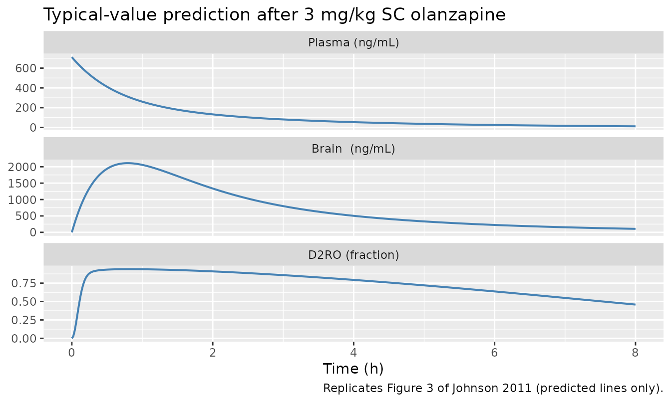
Replicates Figure 3 of Johnson 2011: typical-value plasma olanzapine (top), brain olanzapine (middle), and D2RO (bottom) after 3 mg/kg SC. Concentrations converted to ng/mL for legibility (model native unit is mg/L).
Sensitivity check – IP vs SC bioavailability round-trip
Because IP and SC doses both deposit drug directly into the central compartment (the absorption rate constant was not estimable), a 3 mg/kg IP dose must produce a plasma profile that is FIP-fold (about 0.636) the SC profile under the typical-value model. This is a one-line check that the ROUTE_IP encoding is consistent with the Table III estimate.
sim_3ip <- as.data.frame(rxode2::rxSolve(
  mod_typical,
  make_events(amt_mgkg = 3, route = "IP", tmax = 8, dt = 0.02)
))
#> ℹ omega/sigma items treated as zero: 'etalcl', 'etalfip'

ratio <- max(sim_3ip$Cc) / max(sim_3sc$Cc)
cat(sprintf("IP/SC ratio of max plasma C = %.3f (Table III FIP = 0.636)\n",
            ratio))
#> IP/SC ratio of max plasma C = 0.636 (Table III FIP = 0.636)
stopifnot(abs(ratio - 0.636) < 0.005)
Sensitivity check – brain-to-plasma steady-state ratio
Mass balance across the BBB sets the steady-state brain-to-plasma
total concentration ratio to
fu_plasma / fu_brain = 0.23 / 0.034 = 6.76 (the unbound
concentrations equate across the BBB). After a single bolus this exact
ratio is approached only when the systemic disposition has slowed to the
brain-clearance timescale, so the simulated late-time ratio should
approach (but not equal) 6.76.
Replicating Figure 4 – sensitivity analysis at 3 mg/kg
Figure 4 of Johnson 2011 perturbs Kd (and separately koff, kon) by a factor of 5 above and below the typical value and overlays the resulting D2RO profiles. We re-run the typical-value model with the same factor sweep on Kd to verify that the model produces the same shape: the high-Kd curves saturate later and never reach full occupancy, while the low-Kd curves saturate quickly and stay near 1.
kd_factors <- c(0.2, 1, 5)
sim_kd <- lapply(kd_factors, function(fac) {
  mod_kd <- mod_typical |>
    rxode2::ini(lkd = log(14.7 * fac))
  as.data.frame(rxode2::rxSolve(
    mod_kd,
    make_events(amt_mgkg = 3, route = "SC", tmax = 8, dt = 0.05)
  )) |>
    dplyr::mutate(kd_factor = factor(fac, levels = kd_factors))
}) |>
  dplyr::bind_rows()
#> ℹ change initial estimate of `lkd` to `1.07840958135059`
#> ℹ omega/sigma items treated as zero: 'etalcl', 'etalfip'
#> ℹ change initial estimate of `lkd` to `2.68784749378469`
#> ℹ omega/sigma items treated as zero: 'etalcl', 'etalfip'
#> ℹ change initial estimate of `lkd` to `4.29728540621879`
#> ℹ omega/sigma items treated as zero: 'etalcl', 'etalfip'

ggplot(sim_kd, aes(time, D2RO, colour = kd_factor)) +
  geom_line(linewidth = 0.7) +
  scale_colour_brewer(palette = "Set1",
                      name = "Kd / 14.7 nM") +
  labs(x = "Time (h)", y = "D2RO (fraction)",
       title = "Kd sensitivity at 3 mg/kg SC",
       caption = "Replicates Figure 4 of Johnson 2011 (Kd perturbation panel).")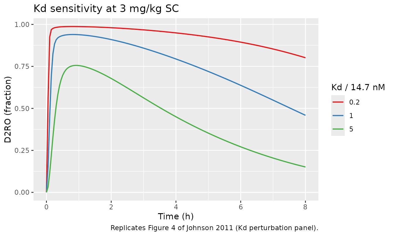
Dose-response at 1 h post-dose (SC)
The TI Pharma dataset spans 0.01-40 mg/kg single doses. The model’s
typical-value D2RO at 1 h post-dose should be sigmoidal in log dose with
the inflection near the dose that produces an unbound brain
concentration equal to Kd / fu_brain. This is a sanity check on the
binding kinetics and unit conversion
(Cbev[nM] = Cbev[mg/L] * 1e6 / MW).
doses <- c(0.01, 0.03, 0.1, 0.3, 1, 3, 10, 30)
ro_1h <- vapply(doses, function(d) {
  sim <- as.data.frame(rxode2::rxSolve(
    mod_typical,
    make_events(amt_mgkg = d, route = "SC", tmax = 1.5, dt = 0.05)
  ))
  sim$D2RO[which.min(abs(sim$time - 1))]
}, numeric(1))
#> ℹ omega/sigma items treated as zero: 'etalcl', 'etalfip'
#> ℹ omega/sigma items treated as zero: 'etalcl', 'etalfip'
#> ℹ omega/sigma items treated as zero: 'etalcl', 'etalfip'
#> ℹ omega/sigma items treated as zero: 'etalcl', 'etalfip'
#> ℹ omega/sigma items treated as zero: 'etalcl', 'etalfip'
#> ℹ omega/sigma items treated as zero: 'etalcl', 'etalfip'
#> ℹ omega/sigma items treated as zero: 'etalcl', 'etalfip'
#> ℹ omega/sigma items treated as zero: 'etalcl', 'etalfip'

dose_resp <- data.frame(dose_mgkg = doses, D2RO_1h = round(ro_1h, 3))
knitr::kable(dose_resp,
caption = "Typical-value D2RO at 1 h post-SC-dose, by dose.")| dose_mgkg | D2RO_1h |
|---|---|
| 0.01 | 0.043 |
| 0.03 | 0.120 |
| 0.10 | 0.323 |
| 0.30 | 0.603 |
| 1.00 | 0.837 |
| 3.00 | 0.939 |
| 10.00 | 0.981 |
| 30.00 | 0.993 |
ggplot(dose_resp, aes(dose_mgkg, D2RO_1h)) +
  geom_point() +
  geom_line() +
  scale_x_log10() +
  scale_y_continuous(limits = c(0, 1)) +
  labs(x = "SC dose (mg/kg, log scale)", y = "D2RO at 1 h (fraction)")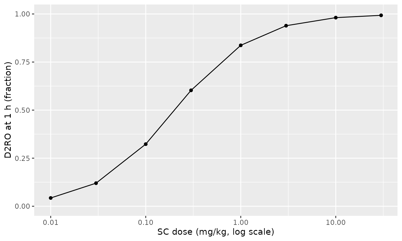
Typical-value D2RO at 1 h after a single SC dose of olanzapine. Steep sigmoid in log dose, ED50 near 0.2 mg/kg SC.
Stochastic predictive check at 3 mg/kg SC
The full model carries between-animal variability on CL (56% CV) and on the IP bioavailability FIP (87% CV; not active for SC doses). Simulating a modest cohort with IIV active and overlaying the resulting D2RO band illustrates how much of the 3 mg/kg SC predictive uncertainty is driven by CL alone (the only IIV term active for SC doses; brain PK and PD parameters are typical-value only because the original dataset had too few brain observations per animal to estimate IAV).
set.seed(20260522L)

n_sim <- 100L
ev_pop <- dplyr::bind_rows(lapply(seq_len(n_sim), function(i) {
  make_events(amt_mgkg = 3, route = "SC", tmax = 8, dt = 0.1, id = i)
}))
stopifnot(!anyDuplicated(unique(ev_pop[, c("id", "time", "evid")])))

sim_pop <- as.data.frame(rxode2::rxSolve(mod, ev_pop))

bands <- sim_pop |>
  dplyr::filter(!is.na(D2RO)) |>
  dplyr::group_by(time) |>
  dplyr::summarise(
    p05 = quantile(D2RO, 0.05),
    p50 = quantile(D2RO, 0.50),
    p95 = quantile(D2RO, 0.95),
    .groups = "drop"
  )

ggplot(bands, aes(time, p50)) +
  geom_ribbon(aes(ymin = p05, ymax = p95), alpha = 0.25, fill = "steelblue") +
  geom_line(linewidth = 0.7, colour = "steelblue") +
  scale_y_continuous(limits = c(0, 1)) +
  labs(x = "Time (h)", y = "D2RO (fraction)",
       title = "Predictive band -- 3 mg/kg SC olanzapine",
       caption = "Median (line) and 5-95% band (ribbon) from 100 simulated rats; IIV on CL only.")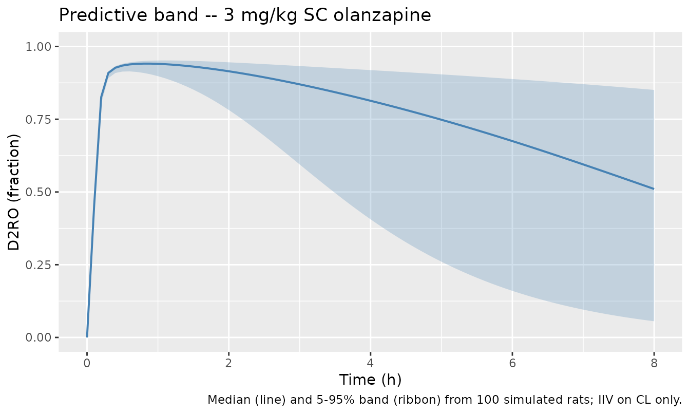
Median plus 5th-95th percentile predictive band for D2RO after 3 mg/kg SC olanzapine, n = 100 simulated rats. The only active IIV for SC dosing is on systemic clearance.
Assumptions and deviations
-
No absorption rate constant. The paper explicitly
states ka could not be estimated, so all routes (IP, SC, IV) dose into
the central compartment directly. This means the simulated peak plasma
concentration is at
t = 0with full bolus amplitude, while real SC and IP absorption is more gradual. AUC and the D2RO timecourse are still well-defined; the peak is an artefact of the chosen structural simplification. - Bmax dropped (reduced model). The final model is Johnson 2011’s reduced PBPKPD (Bmax non-influential per their sensitivity analysis; Tables IV and V show < 1% difference in the binding parameters between the full and reduced fits). The receptor-occupancy ODE is driven by the free brain-extravascular concentration directly, with no separate free / bound striatum compartment.
-
No IIV on brain PK or on the binding kinetics. The
paper estimates IAV only for CL and FIP because the brain dataset had at
most one brain observation per animal; this file mirrors that decision.
The IIV on FIP is encoded via
etalfipand is active only for IP doses (ROUTE_IP = 1). -
SC and IV bioavailability fixed at 1. SC was
estimated to be close to 1 and the paper fixed it; IV is 1 by
definition. The single
ROUTE_IPcovariate flagging IP-vs-not is sufficient because both non-IP routes share the same F. -
Brain-extravascular nM conversion. Appendix 1
writes
CEV [nM] = (A4/V4) / (MW/1000), which is dimensionally consistent only whenA4/V4is reported in ug/L (i.e. NONMEM ran with amounts in ug and volumes in L). This file’s amounts are in mg and volumes in L, so the equivalent dimensionally-correct factor is1e6 / MW. The published kon (= koff / Kd = 0.178 nM^-1 h^-1) is preserved. -
Coupling between plasma and brain compartments. The
paper fit the plasma 2-compartment model alone before fixing those
parameters and fitting the brain submodel sequentially. The packaged
model includes the cerebral-blood-flow coupling
-CLbv * (Cp - Cbv)in the central compartment equation per Appendix 1, so the plasma profile under the full PBPKPD model is mildly lower than under the standalone plasma fit (CLbv / CL = 0.097 of CL, but the loss is nearly cancelled by Cbv approaching Cp at quasi-steady-state). - Multi-strain pooling. Wistar and Sprague-Dawley rats are pooled into a single dataset and the paper reports no strain effect on PK. The model file follows that.
-
checkModelConventions()units warning is the known per-kg false-positive. The package’s convention linter flagsunits$dosing = "mg/kg"andunits$concentration = "mg/L"as “appear dimensionally incompatible” because it compares the literal unit strings rather than per-kg-normalised dimensional consistency. The same warning is emitted forAhlstrom_2010_nicotinicAcid_ratand is the accepted shape for preclinical per-kg models; mg/kg amounts divided by L/kg volumes give mg/L concentrations, which is the convention reported throughout the source paper. - Reference physiology values. Vbv, Vbev, CLbv, fu_plasma, fu_brain are fixed to the literature values cited by the source paper (refs. 18 and 19) and should be re-checked before extrapolating to a non-rat species; the rat-to-human projection in the paper substitutes the human physiology values listed in their Table II.