Cyclosporine (Gao 2022)
Source:vignettes/articles/Gao_2022_cyclosporine.Rmd
Gao_2022_cyclosporine.RmdModel and source
- Citation: Gao X, Bian ZL, Qiao XH, Qian XW, Li J, Shen GM, Miao H, Yu Y, Meng JH, Zhu XH, Jiang JY, Le J, Yu L, Wang HS, Zhai XW. Population Pharmacokinetics of Cyclosporine in Chinese Pediatric Patients With Acquired Aplastic Anemia. Front Pharmacol. 2022;13:933739. doi:10.3389/fphar.2022.933739
- Description: Two-compartment population PK model with first-order absorption for oral cyclosporine A in Chinese children with acquired aplastic anemia (Gao 2022), with fixed allometric body-weight scaling (reference 28 kg) on all clearances and volumes, a linear total-bilirubin effect on CL/F, peripheral volume and intercompartmental clearance fixed from the literature, and log-normal residual error on whole-blood concentrations.
- Article: https://doi.org/10.3389/fphar.2022.933739 (open access)
Population
Gao 2022 pooled 681 sparse whole-blood cyclosporine concentrations from 157 Chinese children (age 1.5-18.8 years, median 7.8; body weight 12.0-91.0 kg, median 27.5) with acquired aplastic anemia treated at two Shanghai hospitals between 2014 and 2021 (Table 1). 59.9% had non-severe, 25.4% severe and 13.4% very severe disease; children who had received a stem-cell transplant were excluded. Oral cyclosporine was started at 5 mg/kg/day in two divided doses and titrated to 5-8 (up to 10) mg/kg/day against a 100-200 ng/mL trough and 300-400 ng/mL peak window. Samples were therapeutic-drug-monitoring peaks (2-4 h post-dose) and pre-dose troughs, measured with the Emit 2000 cyclosporine-specific assay. Median baseline total bilirubin was 10.90 umol/L (range 4.00-70.00). Common co-medications were testosterone undecanoate (70.7%), methylprednisolone (29.9%) and rabbit ATG (29.9%); none was retained as a covariate. The sex distribution is not reported.
The same information is available programmatically via
readModelDb("Gao_2022_cyclosporine")()$population.
Source trace
| Equation / parameter | Value | Source location |
|---|---|---|
lka |
log(1.26) 1/h | Table 2, Ka |
lcl |
log(29.1) L/h | Table 2, CL/F (typical 28-kg child) |
lvc |
log(325) L | Table 2, VC/F |
lq |
fixed(log(3.1)) L/h | Table 2, Q/F “FIX” |
lvp |
fixed(log(262)) L | Table 2, VP/F “FIX” |
e_wt_cl, e_wt_vc
|
fixed 0.75, 1 | Eqs 2-3; Table 2 footnote |
e_tbili_cl |
-0.0107 per umol/L | Table 2, “TBIL on CL (%)” -1.07; footnote equation |
etalcl |
0.0755 (28.0% CV) | Table 2, CV for IIV; log(CV^2 + 1) |
etalvc |
0.326 (62.1% CV) | Table 2, CV for IIV; log(CV^2 + 1) |
expSd |
0.348 | Table 2, sigma (additive on log concentrations) |
| Allometric reference 28 kg | n/a | Methods, Eqs 2-3 (“BWmedian … (28 kg)”) |
| TBIL centring 10.65 umol/L | n/a | Table 2 footnote equation |
| CL equation | n/a | Eq 2 and Table 2 footnote, with 1 + restored (see
below) |
| Two-compartment, first-order absorption ODEs | n/a | Results paragraph 2; Abstract |
| Log-additive residual error | n/a | Methods, Eq 1 paragraph |
Virtual cohorts
Figure 3 of Gao 2022 simulates 1,000 children per body-weight band (10-60 kg) at three fixed total-bilirubin levels. Here each band has 200 children. Panel A is labelled “< 17.1 umol/L” (the upper limit of normal) without a single value; it is simulated at the model’s centring value, 10.65 umol/L. Panels B and C use the printed 25.65 and 34.2 umol/L.
n_per_cell <- 200L
fig3_grid <- tidyr::expand_grid(
  panel = c("A", "B", "C"),
  WT = c(10, 20, 30, 40, 50, 60)
) |>
  dplyr::mutate(
    TBILI = c(A = 10.65, B = 25.65, C = 34.2)[panel],
    cell = dplyr::row_number()
  )

# One steady-state dose of 2.5 mg/kg (5 mg/kg/day split twice daily) and a
# trough observation one dosing interval later.
fig3_events <- fig3_grid |>
  dplyr::slice(rep(seq_len(dplyr::n()), each = n_per_cell)) |>
  dplyr::mutate(id = dplyr::row_number()) |>
  dplyr::reframe(
    dplyr::bind_rows(
      tibble::tibble(
        time = 0, evid = 1L, amt = 2.5 * WT, ss = 1L, ii = 12, cmt = "depot"
      ),
      tibble::tibble(
        time = 12, evid = 0L, amt = 0, ss = 0L, ii = 0, cmt = "central"
      )
    ),
    .by = c(id, panel, WT, TBILI, cell)
  ) |>
  dplyr::arrange(id, time, dplyr::desc(evid))
stopifnot(!anyDuplicated(fig3_events[, c("id", "time", "evid")]))
Simulation
mod <- readModelDb("Gao_2022_cyclosporine")
rxode2::rxSetSeed(20220726)
sim_fig3 <- rxode2::rxSolve(
  mod,
  events = fig3_events,
  keep = c("panel", "WT", "TBILI"),
  maxsteps = 1e6
) |>
  as.data.frame()
#> ℹ parameter labels from comments will be replaced by 'label()'
stopifnot(!anyNA(sim_fig3$Cc))
Replicate published figures
Figure 3: steady-state troughs by body weight and total bilirubin
The published boxes (median and 25th-75th percentiles) were digitised
by the maintainers from the native-resolution Figure 3 image, with the y
axis calibrated on the 0-400 ng/mL gridlines (about 0.75 ng/mL per
pixel). The boxes show exposure without residual error, so the
comparison uses Cc.
fig3_published <- tibble::tribble(
  ~panel, ~WT, ~q25, ~q50, ~q75,
  "A", 10, 48.5, 79.9, 116.4,
  "A", 20, 64.9, 99.3, 142.2,
  "A", 30, 78.0, 117.9, 159.0,
  "A", 40, 88.4, 132.1, 180.6,
  "A", 50, 101.9, 145.5, 196.3,
  "A", 60, 103.7, 154.5, 207.5,
  "B", 10, 70.5, 103.0, 146.3,
  "B", 20, 89.6, 136.6, 187.3,
  "B", 30, 106.7, 157.5, 207.5,
  "B", 40, 126.9, 177.6, 234.3,
  "B", 50, 133.2, 186.6, 239.9,
  "B", 60, 144.8, 201.5, 259.0,
  "C", 10, 84.0, 125.4, 171.6,
  "C", 20, 116.4, 161.2, 217.5,
  "C", 30, 131.0, 176.9, 241.0,
  "C", 40, 147.0, 197.8, 269.4,
  "C", 50, 161.2, 218.7, 282.5,
  "C", 60, 164.9, 231.0, 303.0
)

fig3_sim <- sim_fig3 |>
  dplyr::filter(time == 12) |>
  dplyr::summarise(
    q25 = quantile(Cc, 0.25),
    q50 = quantile(Cc, 0.50),
    q75 = quantile(Cc, 0.75),
    .by = c(panel, WT)
  )

fig3_cmp <- dplyr::inner_join(
  fig3_sim,
  fig3_published,
  by = c("panel", "WT"),
  suffix = c("_sim", "_pub")
) |>
  dplyr::mutate(
    pct_diff_median = 100 * (q50_sim / q50_pub - 1),
    pct_diff_iqr = 100 * ((q75_sim - q25_sim) / (q75_pub - q25_pub) - 1)
  )
stopifnot(nrow(fig3_cmp) == 18L)

fig3_cmp |>
  dplyr::mutate(dplyr::across(dplyr::where(is.numeric), \(x) round(x, 1))) |>
  dplyr::select(
    panel, WT, q50_sim, q50_pub, pct_diff_median, pct_diff_iqr
  ) |>
  dplyr::rename(
    "Panel" = panel,
    "Weight (kg)" = WT,
    "Simulated median (ng/mL)" = q50_sim,
    "Published median (ng/mL)" = q50_pub,
    "Median difference (%)" = pct_diff_median,
    "IQR-width difference (%)" = pct_diff_iqr
  ) |>
knitr::kable(caption = "Steady-state trough, simulated vs. Figure 3.")| Panel | Weight (kg) | Simulated median (ng/mL) | Published median (ng/mL) | Median difference (%) | IQR-width difference (%) |
|---|---|---|---|---|---|
| A | 10 | 76.3 | 79.9 | -4.6 | -0.3 |
| A | 20 | 103.3 | 99.3 | 4.0 | -4.6 |
| A | 30 | 125.1 | 117.9 | 6.1 | 9.5 |
| A | 40 | 141.3 | 132.1 | 7.0 | 8.5 |
| A | 50 | 141.0 | 145.5 | -3.1 | -18.0 |
| A | 60 | 155.0 | 154.5 | 0.3 | 0.8 |
| B | 10 | 98.4 | 103.0 | -4.5 | -6.3 |
| B | 20 | 141.9 | 136.6 | 3.9 | -13.6 |
| B | 30 | 158.7 | 157.5 | 0.8 | -7.5 |
| B | 40 | 171.9 | 177.6 | -3.2 | -10.6 |
| B | 50 | 184.2 | 186.6 | -1.3 | 17.9 |
| B | 60 | 194.9 | 201.5 | -3.3 | -8.4 |
| C | 10 | 124.7 | 125.4 | -0.6 | -8.1 |
| C | 20 | 153.4 | 161.2 | -4.8 | -4.3 |
| C | 30 | 196.9 | 176.9 | 11.3 | -12.1 |
| C | 40 | 209.2 | 197.8 | 5.8 | -4.0 |
| C | 50 | 225.8 | 218.7 | 3.3 | 6.3 |
| C | 60 | 236.9 | 231.0 | 2.6 | -9.0 |
panel_labels <- c(
  A = "(A) TBIL < 17.1 umol/L (sim. 10.65)",
  B = "(B) TBIL = 25.65 umol/L",
  C = "(C) TBIL = 34.2 umol/L"
)
ggplot() +
  geom_boxplot(
    data = sim_fig3 |> dplyr::filter(time == 12),
    aes(x = factor(WT), y = Cc),
    outlier.shape = NA, coef = 0, fill = "grey90"
  ) +
  geom_point(
    data = fig3_published,
    aes(x = factor(WT), y = q50),
    colour = "firebrick", shape = 4, size = 3
  ) +
  geom_errorbar(
    data = fig3_published,
    aes(x = factor(WT), ymin = q25, ymax = q75),
    colour = "firebrick", width = 0.3
  ) +
  facet_wrap(~panel, labeller = labeller(panel = panel_labels)) +
  coord_cartesian(ylim = c(0, 400)) +
  labs(
    x = "Body weight (kg)",
    y = "Cyclosporine trough (ng/mL)",
    caption = paste(
      "Replicates Figure 3 of Gao 2022. Grey boxes: simulated median and IQR;",
      "red: digitised published median and IQR."
    )
  )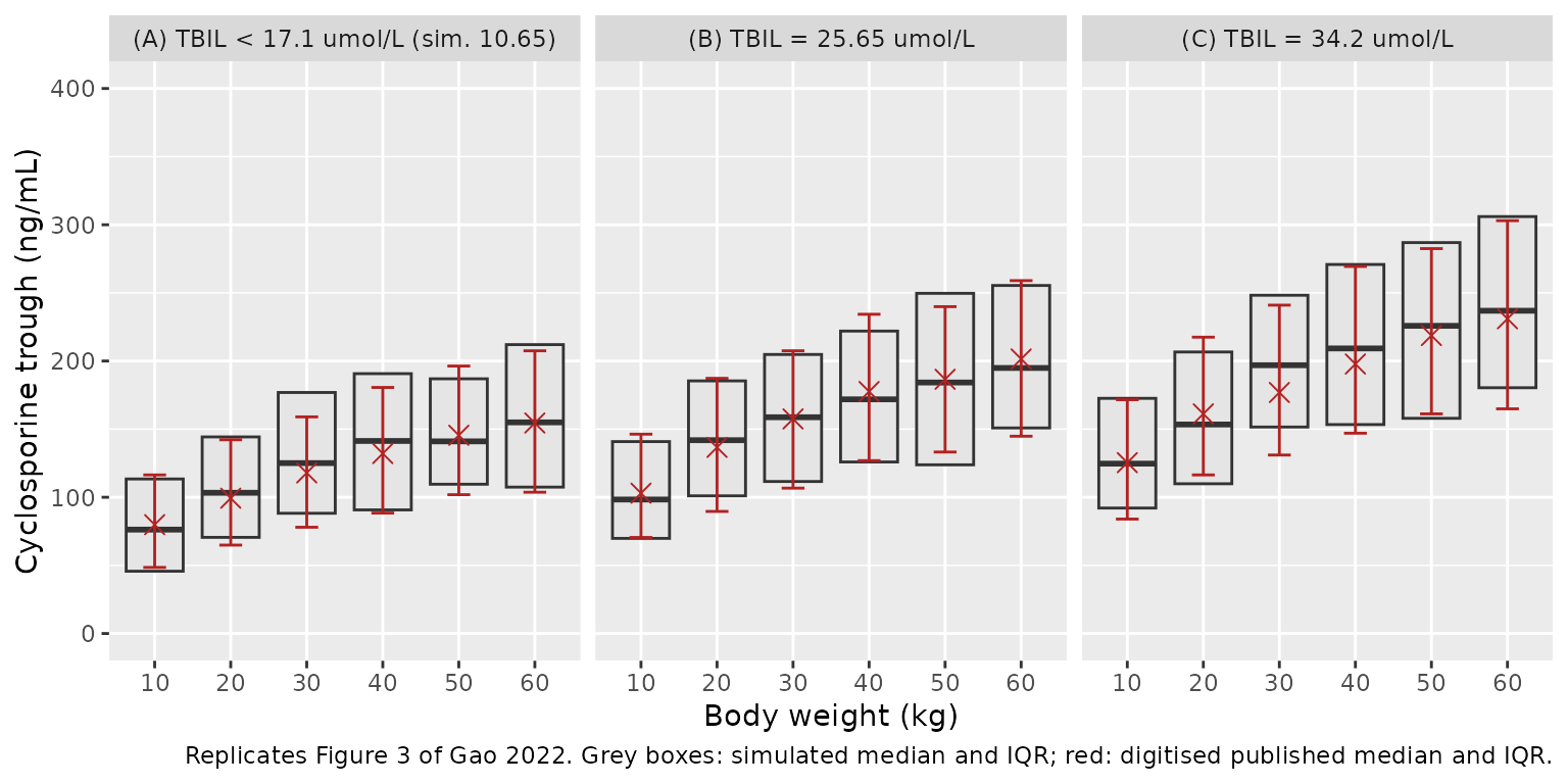
The dose (mg/kg), the clearance, both volumes and the bilirubin slope all set the median trough, and the two IIV variances set the box height. A mis-transcribed value in any of them moves these columns by tens of percent. Each simulated median has a Monte-Carlo SE of about 5% (log-scale SD about 0.55 over 200 children), so the gate is on the centre and the 90th percentile of the 18 cells, never on the worst cell.
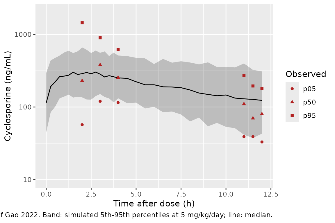
Figure 2: visual predictive check
Gao 2022 Figure 2 is a prediction-corrected VPC of the observed data,
whose doses were titrated between 5 and 10 mg/kg/day. The simulation
below is a qualitative counterpart. It uses 200 children at the starting
regimen of 2.5 mg/kg twice daily, with weight and bilirubin drawn
log-normally around the Table 1 medians, and includes residual error
(sim). The red points are the observed 5th, 50th and 95th
percentiles read by eye from Figure 2, so they are approximate.
set.seed(933739)
n_vpc <- 200L
vpc_subjects <- tibble::tibble(
  id = seq_len(n_vpc),
  WT = pmin(pmax(exp(rnorm(n_vpc, log(27.5), 0.40)), 12), 91),
  TBILI = pmin(pmax(exp(rnorm(n_vpc, log(10.9), 0.45)), 4), 70)
)
vpc_times <- c(seq(0, 4, by = 0.25), seq(4.5, 12, by = 0.5))
vpc_events <- vpc_subjects |>
  dplyr::reframe(
    dplyr::bind_rows(
      tibble::tibble(
        time = 0, evid = 1L, amt = 2.5 * WT, ss = 1L, ii = 12, cmt = "depot"
      ),
      tibble::tibble(
        time = vpc_times, evid = 0L, amt = 0, ss = 0L, ii = 0, cmt = "central"
      )
    ),
    .by = c(id, WT, TBILI)
  ) |>
  dplyr::arrange(id, time, dplyr::desc(evid))

sim_vpc <- rxode2::rxSolve(
  mod,
  events = vpc_events,
  keep = c("WT", "TBILI"),
  maxsteps = 1e6
) |>
  as.data.frame()
stopifnot(!anyNA(sim_vpc$Cc))
fig2_observed <- tibble::tribble(
  ~time, ~p05, ~p50, ~p95,
  2, 57, 230, 1450,
  3, 120, 380, 900,
  4, 115, 255, 620,
  11, 39, 110, 270,
  11.5, 39, 70, 195,
  12, 33, 80, 180
) |>
  tidyr::pivot_longer(-time, names_to = "percentile", values_to = "conc")

sim_vpc |>
  dplyr::summarise(
    p05 = quantile(sim, 0.05),
    p50 = quantile(sim, 0.50),
    p95 = quantile(sim, 0.95),
    .by = time
  ) |>
  ggplot(aes(time)) +
  geom_ribbon(aes(ymin = p05, ymax = p95), alpha = 0.25) +
  geom_line(aes(y = p50)) +
  geom_point(
    data = fig2_observed,
    aes(y = conc, shape = percentile),
    colour = "firebrick"
  ) +
  scale_y_log10(limits = c(10, 2000)) +
  labs(
    x = "Time after dose (h)",
    y = "Cyclosporine (ng/mL)",
    shape = "Observed",
    caption = paste(
      "Compare with Figure 2 of Gao 2022. Band: simulated 5th-95th",
      "percentiles at 5 mg/kg/day; line: median."
    )
  )
PKNCA validation
Gao 2022 reports no NCA table. PKNCA is run over one steady-state
dosing interval of the VPC cohort. The check is cohort-free: each
child’s AUCtau at steady state must equal Dose / CL for that child’s own
clearance (cl in the simulation output).
sim_nca <- sim_vpc |>
  dplyr::filter(!is.na(Cc)) |>
  dplyr::mutate(treatment = "2.5 mg/kg q12h") |>
  dplyr::select(id, time, Cc, treatment)

conc_obj <- PKNCA::PKNCAconc(sim_nca, Cc ~ time | treatment + id)

dose_df <- vpc_events |>
  dplyr::filter(evid == 1) |>
  dplyr::mutate(treatment = "2.5 mg/kg q12h") |>
  dplyr::select(id, time, amt, treatment)
dose_obj <- PKNCA::PKNCAdose(dose_df, amt ~ time | treatment + id)

intervals <- data.frame(
  start = 0,
  end = 12,
  cmax = TRUE,
  tmax = TRUE,
  cmin = TRUE,
  auclast = TRUE
)
nca_res <- PKNCA::pk.nca(
  PKNCA::PKNCAdata(conc_obj, dose_obj, intervals = intervals)
)

nca_wide <- as.data.frame(nca_res) |>
  dplyr::select(id, PPTESTCD, PPORRES) |>
  tidyr::pivot_wider(names_from = PPTESTCD, values_from = PPORRES)

auc_check <- sim_vpc |>
  dplyr::distinct(id, cl, WT) |>
  dplyr::inner_join(nca_wide, by = "id") |>
  dplyr::mutate(
    auc_expected = 1000 * 2.5 * WT / cl,
    pct_diff = 100 * (auclast / auc_expected - 1)
  )
stopifnot(nrow(auc_check) == n_vpc)

auc_check |>
  dplyr::summarise(
    dplyr::across(c(cmax, tmax, cmin, auclast), median)
  ) |>
  dplyr::mutate(dplyr::across(dplyr::everything(), \(x) signif(x, 3))) |>
  dplyr::rename(
    "Cmax,ss (ng/mL)" = cmax,
    "Tmax (h)" = tmax,
    "Cmin,ss (ng/mL)" = cmin,
    "AUCtau,ss (ng*h/mL)" = auclast
  ) |>
knitr::kable(caption = "Median steady-state NCA, 2.5 mg/kg twice daily.")| Cmax,ss (ng/mL) | Tmax (h) | Cmin,ss (ng/mL) | AUCtau,ss (ng*h/mL) |
|---|---|---|---|
| 291 | 2 | 119 | 2460 |
AUCtau and Dose/CL use the same drawn parameters, so the only difference is trapezoidal error on the 0.25-0.5 h grid around the peak. The peak is broad (Ka 1.26 1/h), so that error is a fraction of a percent.
The paper’s Results note that children under 30 kg fall below the 100-200 ng/mL trough window on 5 mg/kg/day. In the Figure 3 replication, the simulated median trough at 10 and 20 kg with normal bilirubin is below 100 ng/mL, which agrees.
Assumptions and deviations
-
Bilirubin equation. The Table 2 footnote prints
CL = CLtypical x ((TBIL - 10.65) x -0.0107), which would make clearance negative at the reference bilirubin. The maintainers restored the missing1 +:CL = CLtypical x (1 - 0.0107 x (TBIL - 10.65)). This matches the text (“a 1.07% reduction per 1 … rise in total bilirubin”), and the Figure 3 replication above reproduces all three bilirubin panels with it. The Abstract and Discussion write “per 1 nmol/L”; Table 1 reports bilirubin in umol/L and the Figure 3 thresholds (17.1, 25.65, 34.2 umol/L) are in umol/L, so the slope is per umol/L. The linear factor reaches zero at TBIL = 104 umol/L, above the cohort maximum of 70 umol/L. The model does not truncate it. - Fixed Q/F and Vp/F. The Results text says Vp/F and Q/F were fixed at “496 and 5 L/h” from Eljebari et al. 2012, while Table 2 prints 262 L and 3.1 L/h “FIX”. Table 2 gives estimates for the typical 28-kg child, and both Table 2 values equal the text values times the same allometric weight ratio (262/496 = 0.528 and 3.1/5 = 0.620 = 0.528^0.75). So the text quotes the literature values at the literature model’s reference weight, and Table 2 quotes them scaled to 28 kg. The Discussion’s total V/F normalised to 70 kg, 1,468 L, equals (325 + 262) x 70/28 = 1,467.5 L, which confirms 262 L. The model uses the Table 2 values.
- IIV scale. The Table 2 footnote gives the IIV CV as “100 x (evariance)1/2”. Read literally this is always above 100%, so the maintainers read it as the log-normal CV, 100 x sqrt(e^variance - 1), and used omega^2 = log(CV^2 + 1). The other reading (CV = 100 x omega) gives omega^2 = 0.0784 and 0.386 for CL/F and Vc/F. Figure 3 cannot tell the two apart: at 1,000 children per band both reproduce the published IQRs to within a few percent. The SIR intervals are percentile intervals, which the scale change does not affect.
-
Residual error. Table 2 labels the value 0.348
“sigma”, and the Methods define the residual variance as sigma^2, so
0.348 is used as the log-scale SD (
lnorm(expSd)). The printed SIR interval (0.356-0.393) does not contain the point estimate and was not used. - Allometric reference. The Methods give the median weight as 28 kg and use it for centring, although Table 1 prints 27.5 kg. The model uses 28 kg.
- Figure 3 panel A has no single bilirubin value (“< 17.1 umol/L”) and is simulated at 10.65 umol/L, the centring value.
- Figure 2 cohort. Individual doses, weights and bilirubin values are not available. The VPC cohort draws weight and bilirubin log-normally around the Table 1 medians, clipped to the Table 1 ranges, and doses everyone at the starting regimen. The observed percentiles were read by eye, so Figure 2 is a qualitative comparison only.
- No erratum or correction notice for Gao 2022 was found in Europe PMC or Crossref as of 2026-10-05.