Tacrolimus (Dunlap 2025)
Source:vignettes/articles/Dunlap_2025_tacrolimus.Rmd
Dunlap_2025_tacrolimus.RmdModel and source
- Citation: Dunlap TC, Zhu J, Weiner DL, Kemper RM, DeVane SC, Ma F, Nguyen V, Coghill JM, Dang V, Grgic T, Jamieson K, Miller J, Myers J, Patel T, Riches M, Serody JS, Trepte M, Vincent BG, Wood WA, Ptachcinski JR, Shaw JR, Weimer E, Armistead PM, Crona DJ. A Tacrolimus Population Pharmacokinetic Model for Adult Allogeneic Hematopoietic Cell Transplant Recipients Provides Clinical Opportunities for Precision Dosing. Clin Pharmacokinet. 2025;64(11):1621-1637. doi:10.1007/s40262-025-01529-w.
- Description: Two-compartment population pharmacokinetic model for oral immediate-release tacrolimus in adult allogeneic hematopoietic cell transplant (allo-HCT) recipients (Dunlap 2025): first-order absorption with bioavailability fixed at 1; allometric (TBW/70 kg) scaling fixed at 0.75 on CL/F and Q/F and at 1 on V1/F and V2/F; exponential CYP3A5 intermediate / normal metabolizer phenotype effect on CL/F (CYP3A5 IM or NM have ~2.14-fold higher CL/F than CYP3A5 PM); exponential reduced-intensity-conditioning effect on CL/F (RIC recipients have ~37% lower CL/F than myeloablative-conditioning recipients); inter-individual variability on V1/F, CL/F, and V2/F; and an additive residual error of 2.51 ng/mL on the linear concentration scale.
- Article: https://doi.org/10.1007/s40262-025-01529-w
Population
The model was developed from 906 oral tacrolimus whole-blood concentrations collected from 290 adult allogeneic hematopoietic cell transplant (allo-HCT) recipients enrolled in two clinical pharmacology studies at the University of North Carolina Medical Center (UNCMC): the retrospective UNC16-1480 cohort (n = 252, single therapeutic-drug-monitoring trough on D-1) and the prospective UNC19-3328 cohort (n = 38, mean 17.2 samples per subject across D-2, D-1, and D0; clinicaltrials.gov NCT04645667). Median (IQR) age was 54 (44, 63) years, total body weight 84 (71, 97) kg, and 43% of subjects were female. Self- reported race was 84% White, 11% Black, and 5% Other. The cohort was predominantly diagnosed with acute leukemia (55%) or MDS (17%); 49% received myeloablative conditioning (MAC) chemotherapy and 51% received reduced- intensity conditioning (RIC). The CYP3A5 metabolizer phenotype distribution was 70% poor metabolizer (PM), 25% intermediate metabolizer (IM), and 5% normal metabolizer (NM), determined by TaqMan diplotype calls of CYP3A51, 3, 6, and 7 alleles (Dunlap 2025 Methods 2.2 and Table 1). All subjects received oral immediate-release tacrolimus at the UNCMC institutional starting dose (0.045 mg/kg twice daily for two days from D-3, then 0.03 mg/kg twice daily) with TDM-driven adjustments retained in the analysis dataset.
The same information is available programmatically via
readModelDb("Dunlap_2025_tacrolimus")$population.
Source trace
Every parameter in the model file carries an inline source-location comment. The table below collects the entries in one place.
| Equation / parameter | Value | Source location |
|---|---|---|
lka (Ka) |
0.50 1/h | Table 2, RCM column, TVKA row (Eq. 4) |
lvc (V1/F at TBW=70 kg) |
150 L | Table 2, RCM column, TVV1/F row (Eq. 5) |
lcl (CL/F at TBW=70 kg, PM, MAC) |
23 L/h | Table 2, RCM column, TVCL/F row (Eq. 6) |
lvp (V2/F at TBW=70 kg) |
1153 L | Table 2, RCM column, TVV2/F row (Eq. 7) |
lq (Q/F at TBW=70 kg) |
43 L/h | Table 2, RCM column, TVQ/F row (Eq. 8) |
e_wt_cl_q (allometric exponent on CL/F and Q/F) |
0.75 (FIX) | Table 2, RCM column, TVCL/F~TBW and TVQ/F~TBW rows |
e_wt_vc_vp (allometric exponent on V1/F and V2/F) |
1 (FIX) | Table 2, RCM column, TVV1/F~TBW and TVV2/F~TBW rows |
e_cyp3a5_expr_cl (CYP3A5 IM or NM factor on CL/F) |
2.14 [1.67, 2.74] | Table 2, RCM column, TVCL/F~CYP3A5 IM or NM row |
e_hct_cond_ric_cl (RIC factor on CL/F) |
0.63 [0.51, 0.77] | Table 2, RCM column, TVCL/F~RIC row |
| IIV V1/F (omega^2 = log(0.95^2 + 1) = 0.65823) | 95% CV | Table 2, RCM column, IIV V1/F row |
| IIV CL/F (omega^2 = log(0.55^2 + 1) = 0.26282) | 55% CV | Table 2, RCM column, IIV CL/F row |
| IIV V2/F (omega^2 = log(0.66^2 + 1) = 0.36185) | 66% CV | Table 2, RCM column, IIV V2/F row |
| Additive residual error | 2.51 ng/mL | Table 2, RCM column, Additive RUV row (Eq. 9; Methods 2.3) |
| Bioavailability F | 1 (fixed) | Methods 2.3 (allometry fixed-to-theory paragraph) |
| Reference subject | 70 kg, CYP3A5 PM, MAC | Section 3.2 (“a 70 kg CYP3A5 PM subject receiving MAC”) |
| Two-cmt, first-order oral absorption | – | Section 3.2 first paragraph; Eqs. 4-9 |
Virtual cohort
The published dataset is not openly available, so the virtual cohort below mirrors the demographics in Dunlap 2025 Table 1 and the four clinically distinct (CYP3A5 phenotype) x (conditioning intensity) sub-groups used in the paper’s Figures 3 and 6.
set.seed(20250812)

n_per_subgroup <- 100L

make_cohort <- function(n, cyp3a5_expr, hct_cond_ric, label, id_offset = 0L) {
  tibble(
    id          = id_offset + seq_len(n),
    WT          = exp(rnorm(n, mean = log(84), sd = 0.20)),  # TBW median 84 kg, IQR 71-97
    CYP3A5_EXPR = cyp3a5_expr,
    HCT_COND_RIC    = hct_cond_ric,
    subgroup    = label
  )
}

# Four sub-groups -- IDs are disjoint across panels (Dunlap 2025 Figure 3C
# layout: PM/RIC, PM/MAC, IM_or_NM/RIC, IM_or_NM/MAC).
demo <- bind_rows(
  make_cohort(n_per_subgroup, cyp3a5_expr = 0L, hct_cond_ric = 1L,
              label = "PM, RIC",       id_offset = 0L * n_per_subgroup),
  make_cohort(n_per_subgroup, cyp3a5_expr = 0L, hct_cond_ric = 0L,
              label = "PM, MAC",       id_offset = 1L * n_per_subgroup),
  make_cohort(n_per_subgroup, cyp3a5_expr = 1L, hct_cond_ric = 1L,
              label = "IM or NM, RIC", id_offset = 2L * n_per_subgroup),
  make_cohort(n_per_subgroup, cyp3a5_expr = 1L, hct_cond_ric = 0L,
              label = "IM or NM, MAC", id_offset = 3L * n_per_subgroup)
)
stopifnot(!anyDuplicated(demo$id))
Simulation
Two regimens are simulated. The first follows the UNCMC institutional dosing protocol used in the paper (0.045 mg/kg BID from D-3 for the first four doses, 0.03 mg/kg BID thereafter; Dunlap 2025 Methods 2.2). The second is the RCM-derived recommendation that was identified as the minimum acceptable increase relative to the institutional protocol for each sub-group (Dunlap 2025 Table 3): no change for PM/RIC, +50% for PM/MAC, +100% for IM-or-NM/RIC, and 0.06 mg/kg three times daily for IM-or-NM/MAC.
build_events <- function(demo, regimen = c("UNCMC", "RCM"), sim_hours = 96) {
  regimen <- match.arg(regimen)

  # Doses are administered on a 12-hour cycle (or 8-hour cycle for the TID
  # IM-or-NM/MAC arm of the RCM strategy). Time origin t=0 is the first
  # dose at D-3, so D0 trough corresponds to t=72 h.
  #
  # In the UNCMC protocol the first 4 doses (covering D-3 and D-2) are
  # 0.045 mg/kg BID and the remaining doses (D-1 and D0) are 0.03 mg/kg BID.
  # In the RCM-derived strategy doses are scaled by sub-group; the IM-or-NM/MAC
  # sub-group switches to 0.06 mg/kg TID.
  per_subject_doses <- function(row) {
    if (regimen == "UNCMC") {
      times <- seq(0, sim_hours - 1, by = 12)
      doses <- ifelse(times < 48,
                      0.045 * row$WT,
                      0.030 * row$WT)
    } else {
      # RCM-derived strategy
      mult <- switch(row$subgroup,
                     "PM, RIC"        = 1.00,
                     "PM, MAC"        = 1.50,
                     "IM or NM, RIC"  = 2.00,
                     "IM or NM, MAC"  = 1.00)  # MAC IM/NM uses TID schedule, see below
      if (row$subgroup == "IM or NM, MAC") {
        times <- seq(0, sim_hours - 1, by = 8)
        doses <- rep(0.06 * row$WT, length(times))
      } else {
        times <- seq(0, sim_hours - 1, by = 12)
        doses <- ifelse(times < 48,
                        0.045 * mult * row$WT,
                        0.030 * mult * row$WT)
      }
    }
    tibble(id = row$id, time = times, amt = doses,
           evid = 1L, cmt = "depot",
           WT = row$WT, CYP3A5_EXPR = row$CYP3A5_EXPR,
           HCT_COND_RIC = row$HCT_COND_RIC, subgroup = row$subgroup)
  }

  doses_df <- do.call(rbind, lapply(seq_len(nrow(demo)),
                                    function(i) per_subject_doses(demo[i, ])))

  # Observation grid: every 30 min for D0 (t=72 to t=84) to characterise the
  # post-dose profile, plus pre-dose troughs at t=24 (D-2), t=48 (D-1),
  # and t=72 (D0).
  obs_times <- sort(unique(c(24, 48, seq(72, 84, by = 0.5))))
  obs <- demo |>
    select(id, WT, CYP3A5_EXPR, HCT_COND_RIC, subgroup) |>
    tidyr::crossing(time = obs_times) |>
    mutate(amt = NA_real_, evid = 0L, cmt = NA_character_)

  bind_rows(doses_df, obs) |>
    arrange(id, time, desc(evid))
}

events_uncmc <- build_events(demo, regimen = "UNCMC")
events_rcm   <- build_events(demo, regimen = "RCM")
mod <- rxode2::rxode2(readModelDb("Dunlap_2025_tacrolimus"))
#> ℹ parameter labels from comments will be replaced by 'label()'

sim_uncmc <- rxode2::rxSolve(
  mod, events = events_uncmc,
  keep   = c("subgroup")
) |> as.data.frame()

sim_rcm <- rxode2::rxSolve(
  mod, events = events_rcm,
  keep   = c("subgroup")
) |> as.data.frame()

# Deterministic typical-value run for the no-IIV comparisons.
mod_typical <- mod |> rxode2::zeroRe()
sim_uncmc_typ <- rxode2::rxSolve(mod_typical, events = events_uncmc,
                                 keep = c("subgroup")) |> as.data.frame()
#> ℹ omega/sigma items treated as zero: 'etalvc', 'etalcl', 'etalvp'
#> Warning: multi-subject simulation without without 'omega'
Replicate published figures
Figure 3 – D0 trough distribution by sub-group under the UNCMC protocol
Dunlap 2025 Figure 3C shows the observed steady-state D0 trough concentration distribution across the four (CYP3A5 phenotype) x (conditioning intensity) sub-groups under the current UNCMC dosing protocol. The simulated trough at t = 72 h (D0 morning, immediately before the next dose) reproduces the qualitative gradient: PM/RIC sits highest (often above the 5-10 ng/mL ITR), PM/MAC sits at the lower end of the ITR, and IM-or-NM sub-groups sit predominantly below the ITR.
fig3_data <- sim_uncmc |>
  filter(time == 72) |>
  mutate(subgroup = factor(subgroup,
                           levels = c("PM, RIC", "PM, MAC",
                                      "IM or NM, RIC", "IM or NM, MAC")))

ggplot(fig3_data, aes(subgroup, Cc)) +
  annotate("rect", xmin = -Inf, xmax = Inf, ymin = 5, ymax = 10,
           alpha = 0.25, fill = "grey60") +
  geom_boxplot(outlier.size = 0.7) +
  scale_y_continuous(limits = c(0, 30)) +
  labs(x = NULL,
       y = "Simulated D0 trough tacrolimus (ng/mL)",
       caption = "Replicates Figure 3C of Dunlap 2025.")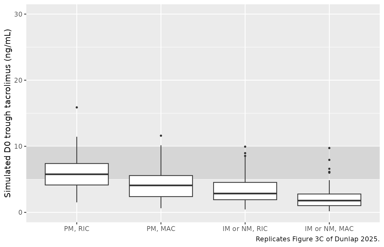
Replicates Figure 3C of Dunlap 2025: simulated D0 trough tacrolimus concentration distribution by (CYP3A5 metabolizer phenotype) x (conditioning regimen intensity) under the UNCMC institutional dosing protocol. Shaded band is the 5-10 ng/mL UNCMC institutional target range.
Figure 5 – D0 dosing-interval pcVPC for the overall cohort
Dunlap 2025 Figure 5 shows a prediction-corrected VPC of the D0 dosing interval (~12 h post the morning D0 dose) overlaid on observed concentrations. The simulated VPC below shows the dose-normalised D0 dosing-interval profile (percentiles 5/50/95) for the full virtual cohort under the UNCMC protocol.
fig5_data <- sim_uncmc |>
  filter(time >= 72, time <= 84) |>
  mutate(time_after_dose = time - 72)

fig5_summary <- fig5_data |>
  group_by(time_after_dose) |>
  summarise(Q05 = quantile(Cc, 0.05, na.rm = TRUE),
            Q50 = quantile(Cc, 0.50, na.rm = TRUE),
            Q95 = quantile(Cc, 0.95, na.rm = TRUE),
            .groups = "drop")

ggplot(fig5_summary, aes(time_after_dose, Q50)) +
  geom_ribbon(aes(ymin = Q05, ymax = Q95), alpha = 0.25, fill = "steelblue") +
  geom_line(linewidth = 0.7) +
  scale_y_log10() +
  scale_x_continuous(breaks = seq(0, 12, by = 4)) +
  labs(x = "Time after D0 dose (h)",
       y = "Tacrolimus concentration (ng/mL)",
       caption = "Replicates Figure 5 of Dunlap 2025.")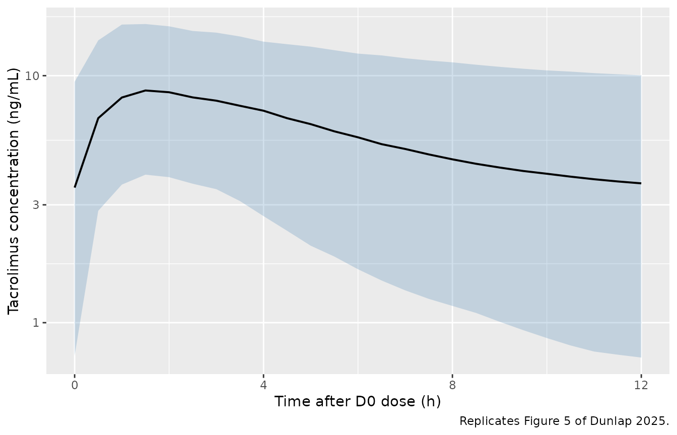
Replicates Figure 5 of Dunlap 2025: simulated tacrolimus concentration vs. time after the D0 dose, percentiles 5/50/95 across all sub-groups, under the UNCMC institutional dosing protocol.
Figure 6 / Table 4 – D0 trough under UNCMC vs. RCM-derived dosing
Dunlap 2025 Figure 6 (and Table 4) compares the population-level D0 trough distribution under the current UNCMC dosing strategy and under the RCM model- derived dosing strategy. The model-derived strategy is expected to shift the overall distribution upward into the 5-10 ng/mL ITR.
fig6_data <- bind_rows(
  sim_uncmc |> filter(time == 72) |> mutate(strategy = "UNCMC protocol"),
  sim_rcm   |> filter(time == 72) |> mutate(strategy = "RCM-derived")
) |>
  mutate(strategy = factor(strategy,
                           levels = c("UNCMC protocol", "RCM-derived")))

ggplot(fig6_data, aes(strategy, Cc)) +
  annotate("rect", xmin = -Inf, xmax = Inf, ymin = 5, ymax = 10,
           alpha = 0.25, fill = "grey60") +
  geom_boxplot(outlier.size = 0.7) +
  scale_y_continuous(limits = c(0, 30)) +
  labs(x = NULL,
       y = "Simulated D0 trough tacrolimus (ng/mL)",
       caption = "Replicates Figure 6 / Table 4 of Dunlap 2025.")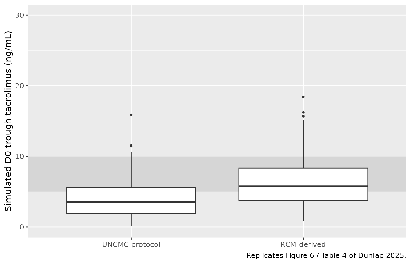
Replicates Figure 6 / Table 4 of Dunlap 2025: simulated D0 trough tacrolimus concentration distribution under the current UNCMC institutional protocol vs. the RCM-derived dosing strategy. Shaded band is the 5-10 ng/mL ITR. Simulated medians fall within the ITR for the model-derived strategy.
PKNCA validation
A standard NCA over the D0 dosing interval (12 h after the D0 morning dose under the UNCMC protocol) gives Cmax, Tmax, and AUC0-12 by sub-group. The PKNCA formula carries the (CYP3A5 phenotype) x (conditioning intensity) grouping so the per-sub-group Cmax can be compared against the paper’s overall safety constraint Cmax limit (24.2 ng/mL, Methods 2.6).
nca_window <- sim_uncmc |>
  filter(time >= 72, time <= 84) |>
  mutate(time_after_dose = time - 72) |>
  select(id, time = time_after_dose, Cc, subgroup)

dose_df <- demo |>
  mutate(time = 0, amt = 0.030 * WT) |>
  select(id, time, amt, subgroup)

conc_obj <- PKNCA::PKNCAconc(nca_window, Cc ~ time | subgroup + id)
dose_obj <- PKNCA::PKNCAdose(dose_df,    amt ~ time | subgroup + id)

intervals <- data.frame(start = 0, end = 12,
                        cmax = TRUE, tmax = TRUE, auclast = TRUE,
                        cmin = TRUE, ctrough = TRUE)

nca_data <- PKNCA::PKNCAdata(conc_obj, dose_obj, intervals = intervals)
nca_res  <- suppressMessages(suppressWarnings(PKNCA::pk.nca(nca_data)))
nca_summary <- summary(nca_res)
knitr::kable(nca_summary,
caption = "D0 dosing-interval NCA on the simulated cohort under the UNCMC institutional protocol (12 h interval).")| start | end | subgroup | N | auclast | cmax | cmin | tmax | ctrough |
|---|---|---|---|---|---|---|---|---|
| 0 | 12 | IM or NM, MAC | 100 | 41.2 [52.5] | 6.33 [39.9] | 1.56 [94.1] | 2.00 [0.500, 3.00] | 1.60 [94.8] |
| 0 | 12 | IM or NM, RIC | 100 | 61.0 [44.4] | 8.18 [36.5] | 2.78 [70.3] | 2.00 [0.500, 4.00] | 2.89 [71.1] |
| 0 | 12 | PM, MAC | 100 | 75.6 [42.4] | 9.56 [36.0] | 3.77 [62.0] | 2.00 [1.00, 3.00] | 3.94 [62.5] |
| 0 | 12 | PM, RIC | 100 | 99.8 [42.4] | 11.7 [37.2] | 5.44 [61.1] | 2.00 [0.500, 4.00] | 5.75 [61.0] |
Comparison against published NCA
Dunlap 2025 does not report a Cmax / AUC NCA table for the analysis cohort (the paper’s primary endpoint is the D0 trough concentration). Instead, Methods 2.6 cites a safety constraint that the predicted Cmax should not exceed 24.2 ng/mL (the average Cmax observed at the FDA-label oral tacrolimus 0.3 mg/kg/day dose in adult renal-transplant recipients). The simulated D0 Cmax across the four sub-groups under the UNCMC protocol is well below that threshold, consistent with the paper’s safety-constraint analysis.
cmax_summary <- sim_uncmc |>
  filter(time >= 72, time <= 84) |>
  group_by(subgroup, id) |>
  summarise(cmax_subj = max(Cc), .groups = "drop") |>
  group_by(subgroup) |>
  summarise(cmax_median = median(cmax_subj),
            cmax_p95    = quantile(cmax_subj, 0.95),
            .groups = "drop")
cmax_summary |>
  dplyr::rename(
    "Sub-group"                                 = subgroup,
    "Simulated D0 Cmax median (ng/mL)"          = cmax_median,
    "Simulated D0 Cmax 95th percentile (ng/mL)" = cmax_p95
  ) |>
  knitr::kable(
             digits = 2,
caption = "Per-sub-group D0 Cmax distribution under the UNCMC protocol; compare against the Dunlap 2025 Methods 2.6 safety constraint of 24.2 ng/mL.")| Sub-group | Simulated D0 Cmax median (ng/mL) | Simulated D0 Cmax 95th percentile (ng/mL) |
|---|---|---|
| IM or NM, MAC | 6.40 | 11.82 |
| IM or NM, RIC | 8.08 | 14.86 |
| PM, MAC | 9.84 | 15.63 |
| PM, RIC | 11.70 | 20.46 |
Assumptions and deviations
- Inter-occasion variability is not modelled. Dunlap 2025 Methods 2.3 describes IIV on PK parameters with a normal distribution of mean zero and variance omega^2; the paper does not report an IOV component in the RCM. The model file therefore implements only IIV on V1/F, CL/F, and V2/F.
- Off-diagonal IIV correlations are set to zero. Dunlap 2025 Table 2 reports IIV %CV for each PK parameter but does not publish the variance-covariance matrix’s off-diagonal elements. The model uses a diagonal IIV block.
- Race / ethnicity is not a model covariate. Dunlap 2025 Table 1 reports race for descriptive purposes (84% White, 11% Black, 5% Other) but the RCM does not include a race covariate. The validation cohort therefore does not stratify by race.
- POR genotype effect is not retained. The full covariate model evaluated POR 1/28 and POR 28/28 effects on CL/F, but neither met the ROPE-based clinical-significance criterion (Dunlap 2025 Section 3.2 / Figure 2A) and they were dropped from the RCM. The packaged model therefore omits POR.
- CYP3A5 IM and NM are pooled as a single binary indicator. Dunlap 2025 Section 3.2 explains that estimating separate TVCL/F~IM and TVCL/F~NM effects in the FCM produced overlapping confidence intervals and that the RCM was simplified to a single TVCL/F~(IM or NM) effect for parsimony and to align with the CPIC dosing recommendations that do not differentiate IM from NM. The model file follows this final RCM choice.
- TBW is used directly without categorisation. The paper reports a Monte Carlo sensitivity analysis of the dosing recommendations at TBW values of 50, 75, 100, and 125 kg (Methods 2.6); the packaged model uses the continuous TBW input and reproduces sub-group differences via the (TBW/70)^0.75 allometric form on CL/F (and Q/F) and (TBW/70)^1 on V1/F (and V2/F).
-
Reference covariate values preserved literally.
Dunlap 2025 reports typical PK parameter values for a 70 kg CYP3A5 PM
subject receiving MAC (Section 3.2). The model file uses these values
verbatim and applies the RCM covariate factors
(
exp(theta)^indicator) on top, reproducing Equations 4-9 directly. -
Bioavailability fixed at 1. Per Dunlap 2025 Methods
2.3, F was not estimated; CL/F, V1/F, V2/F, and Q/F are apparent values
inseparable from F. The model file does not parameterise
lfdepot. - Simulated cohort size. The vignette uses 100 subjects per (CYP3A5 phenotype) x (conditioning intensity) sub-group (400 total), small enough to render the vignette in well under 5 minutes but large enough to give stable percentiles for the per-sub-group trough distributions in Figures 3, 5, and 6.