Tacrolimus, once-daily extended release (Fernandez-Alarcon 2024)
Source:vignettes/articles/FernandezAlarcon_2024_tacrolimus.Rmd
FernandezAlarcon_2024_tacrolimus.RmdModel and source
- Citation: Fernandez-Alarcon B, Nolberger O, Vidal-Alabro A, Rigo-Bonnin R, Grinyo JM, Melilli E, Montero N, Manonelles A, Coloma A, Fava A, Codina S, Cruzado JM, Colom H, Lloberas N. Guiding the starting dose of the once-daily formulation of tacrolimus in ‘de novo’ adult renal transplant patients: a population approach. Front Pharmacol. 2024;15:1456565. doi:10.3389/fphar.2024.1456565.
- Description: Two-compartment population PK model for once-daily extended-release tacrolimus (Advagraf) in de novo adult kidney transplant recipients during the first 15 days post-transplant (Fernandez-Alarcon 2024), with first-order absorption (ka fixed at 2 1/h) after a lag time and linear elimination. Apparent clearance CL/F depends on recipient CYP3A5 expresser status (non-expressers 0.666-fold) and decreases linearly with age above 60 years; CL/F, CLD/F and Vc/F are allometrically scaled to 70 kg body weight. Disposition parameters refer to whole-blood concentrations standardized to a hematocrit of 45%; the predicted whole-blood concentration is the standardized concentration times HCT/45. Between-subject variability on CL/F and Vc/F and a proportional residual error.
- Article: Front Pharmacol 2024;15:1456565
mod <- readModelDb("FernandezAlarcon_2024_tacrolimus")
mod_typical <- rxode2::zeroRe(mod)
#> ℹ parameter labels from comments will be replaced by 'label()'
Population
Fernandez-Alarcon 2024 analysed 1,067 whole-blood tacrolimus concentrations from 138 de novo adult kidney transplant recipients treated at a single Spanish centre (Hospital Universitari de Bellvitge, Barcelona) between 2012 and 2022. All received the once-daily extended-release formulation (Advagraf) from 24 h after transplantation at 0.1 mg/kg/day, titrated to a whole-blood trough of 5-10 ng/mL, together with mycophenolic acid and corticosteroids. Twenty-nine patients had a full 24-h profile on day 5 post-transplant (pre-dose and 0.5, 1, 2, 4, 8, 12, 20 and 24 h) plus troughs on days 10 and 15; the remaining 109 had troughs on days 5, 10 and 15.
Baseline characteristics (Table 1, median and range): age 54 years
(19-82), body weight 70.5 kg (44.0-109.0), BMI 25.6 kg/m^2 (17.2-36.2),
fat-free mass 51.9 kg (30.5-73.9); 90 male and 48 female. CYP3A5
genotype was *1/*1 in 3 (2.2%), *1/*3 in 17
(12.3%) and *3/*3 in 118 (85.5%) patients; CYP3A4
*1/*22 in 12 (8.6%). Hematocrit was low early after
transplantation and rose over the study (Table 2): median 29.7% on day
5, 31.3% on day 10 and 32.9% on day 15 (range 20.9-46.6%).
The same information is available programmatically via the model’s
population metadata
(readModelDb("FernandezAlarcon_2024_tacrolimus")()$population).
Source trace
| Element | Value | Source location |
|---|---|---|
| Structure: 2-compartment, first-order absorption with lag time, linear elimination | – | Results 3.2; Methods 2.6.1 |
lcl (CL/F, 70-kg CYP3A5*1 carrier, age <= 60 y) |
26.5 L/h | Table 4, theta1 |
e_cyp3a5_nonexpr_cl (CL/F multiplier, CYP3A5*1
non-carrier) |
0.666 | Table 4, theta2 and footnote |
e_age_cl (CL/F decrease per year of age when age >
60 y) |
0.0562 L/h/y | Table 4, theta3; Equation 3 |
CL/F equation
(theta1 * theta2 - theta3 * AGE * agecat) * (BW/70)^0.75
|
– | Table 4 header row and footnote; Equation 3 |
lvc (Vc/F, 70 kg) |
327 L | Table 4 |
lvp (Vp/F, not scaled) |
298 L | Table 4 |
lq (CLD/F, 70 kg) |
51.9 L/h | Table 4 |
| Allometric exponents 0.75 (CL/F, CLD/F) and 1 (Vc/F), fixed | – | Table 4 footnote |
lka (Ka, fixed) |
2.0 1/h | Table 4; Results 3.2 |
ltlag (lag time) |
0.341 h | Table 4 |
| F = 1 | – | Methods 2.6.1 |
etalcl |
32.1% CV | Table 4 |
etalvc |
48.2% CV | Table 4 |
propSd |
28.2% | Table 4; Results 3.2 (“modeled as proportional”) |
| Whole-blood concentrations standardized to hematocrit 45% | Cc = Cstd * HCT / 45 |
Methods 2.6.2; Results 3.2 |
Virtual cohort
Observed data are not public. The cohort below mirrors the Monte Carlo design of the paper’s Figures 3 and 4: 70-kg patients, CYP3A5*1 carriers and non-carriers, aged 50 years (any age of 60 or younger gives the same CL/F) or 80 years, with hematocrit drawn uniformly within the paper’s three bands (22-29%, 30-39%, 40-49%). Every subject receives 5 mg once daily from time 0; day 5 of treatment is the fifth dosing interval (96-120 h). Twelve arms of 100 subjects each are simulated. The model is linear in dose, so the exposures at 5.5-7.5 mg in the figure replications are the 5-mg results multiplied by dose / 5.
set.seed(20241004)
rxode2::rxSetSeed(20241004)

n_per_arm <- 100L
dose_mg <- 5
tau <- 24
n_doses <- 5L
t_start <- tau * (n_doses - 1L)
obs_times <- c(seq(t_start, t_start + 2, by = 0.25), seq(t_start + 3, t_start + tau, by = 1))

hct_bands <- tibble::tribble(
  ~hct_band,   ~hct_lo, ~hct_hi,
  "0.22-0.29", 22,      29.9,
  "0.30-0.39", 30,      39.9,
  "0.40-0.49", 40,      49
)

arms <- tidyr::expand_grid(
  CYP3A5_EXPR = c(1, 0),
  AGE = c(50, 80),
  hct_band = hct_bands$hct_band
) |>
  left_join(hct_bands, by = "hct_band") |>
  mutate(
    arm = row_number(),
    genotype = ifelse(CYP3A5_EXPR == 1, "CYP3A5*1 carriers", "CYP3A5*1 non-carriers"),
    age_group = ifelse(AGE > 60, "80 years", "<=60 years")
  )

subjects <- arms |>
  slice(rep(seq_len(n()), each = n_per_arm)) |>
  mutate(
    id = row_number(),
    WT = 70,
    HCT = runif(n(), hct_lo, hct_hi)
  )

doses <- subjects |>
  tidyr::expand_grid(time = tau * (seq_len(n_doses) - 1L)) |>
  mutate(amt = dose_mg, evid = 1L, cmt = "depot")
obs <- subjects |>
  tidyr::expand_grid(time = obs_times) |>
  mutate(amt = NA_real_, evid = 0L, cmt = "central")
events <- bind_rows(doses, obs) |>
  arrange(id, time, desc(evid)) |>
  select(id, time, amt, evid, cmt, WT, AGE, CYP3A5_EXPR, HCT, arm)

stopifnot(dplyr::n_distinct(events$id) == nrow(arms) * n_per_arm)
Simulation
sim <- rxode2::rxSolve(mod, events = events, keep = "arm") |>
  as.data.frame() |>
  left_join(arms |> select(arm, genotype, age_group, hct_band), by = "arm")
#> ℹ parameter labels from comments will be replaced by 'label()'

stopifnot(dplyr::n_distinct(sim$id) == nrow(arms) * n_per_arm)
Typical-value day-5 profiles
typ_events <- tidyr::expand_grid(
  CYP3A5_EXPR = c(1, 0),
  AGE = c(50, 80)
) |>
  mutate(id = row_number(), WT = 70, HCT = 45)
typ_ev <- bind_rows(
  typ_events |> tidyr::expand_grid(time = tau * (seq_len(n_doses) - 1L)) |>
    mutate(amt = dose_mg, evid = 1L, cmt = "depot"),
  typ_events |> tidyr::expand_grid(time = obs_times) |>
    mutate(amt = NA_real_, evid = 0L, cmt = "central")
) |>
  arrange(id, time, desc(evid))

sim_typ <- rxode2::rxSolve(mod_typical, events = typ_ev) |>
  as.data.frame() |>
  mutate(
    genotype = ifelse(CYP3A5_EXPR == 1, "CYP3A5*1 carriers", "CYP3A5*1 non-carriers"),
    age_group = ifelse(AGE > 60, "80 years", "<=60 years")
  )
#> ℹ omega/sigma items treated as zero: 'etalcl', 'etalvc'
#> Warning: multi-subject simulation without without 'omega'

ggplot(sim_typ, aes(time - t_start, Cc, colour = age_group)) +
  geom_line(linewidth = 0.8) +
  facet_wrap(~genotype) +
  geom_hline(yintercept = c(5, 10), linetype = "dashed", colour = "blue") +
  labs(
    x = "Time after the day-5 dose (h)",
    y = "Whole-blood tacrolimus (ng/mL)",
    colour = "Age"
  )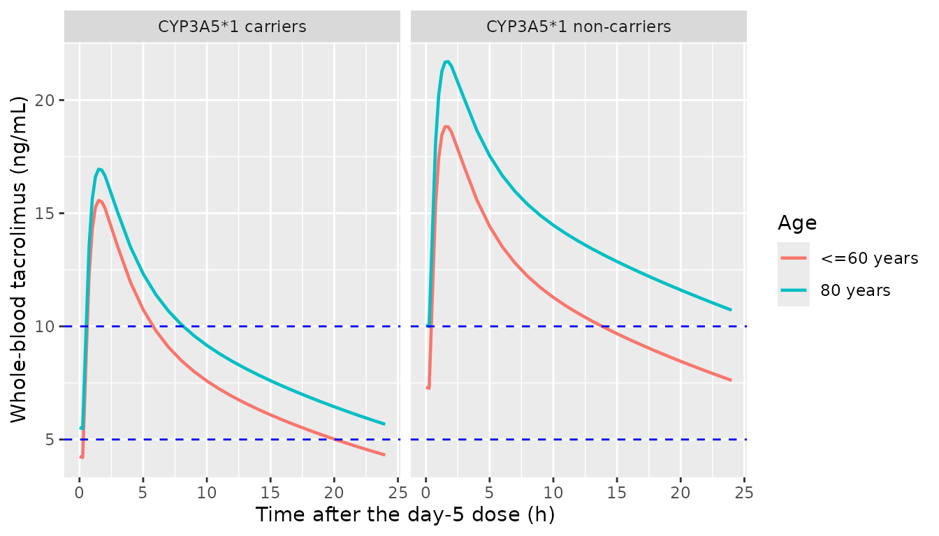
Typical-value (no between-subject variability) whole-blood profiles over the fifth dosing interval of 5 mg once daily at a hematocrit of 45%, by CYP3A5 genotype and age.
PKNCA validation
Exposure on day 5 is computed with PKNCA over the fifth dosing
interval. The treatment grouping variable is the simulated arm (genotype
x age x hematocrit band). cmin over that interval is the
pre-dose trough of the day-5 dose (with the 0.34-h lag the concentration
keeps falling for a few minutes after the dose).
sim_nca <- sim |>
  dplyr::filter(!is.na(Cc)) |>
  dplyr::select(id, time, Cc, arm)

dose_df <- events |>
  dplyr::filter(evid == 1) |>
  dplyr::select(id, time, amt, arm)

conc_obj <- PKNCA::PKNCAconc(sim_nca, Cc ~ time | arm + id, concu = "ng/mL", timeu = "h")
dose_obj <- PKNCA::PKNCAdose(dose_df, amt ~ time | arm + id, doseu = "mg")
intervals <- data.frame(
  start = t_start,
  end = t_start + tau,
  cmax = TRUE,
  tmax = TRUE,
  cmin = TRUE,
  auclast = TRUE
)
nca_res <- PKNCA::pk.nca(PKNCA::PKNCAdata(conc_obj, dose_obj, intervals = intervals))

nca_ind <- as.data.frame(nca_res$result) |>
  dplyr::select(id, arm, PPTESTCD, PPORRES) |>
  tidyr::pivot_wider(names_from = PPTESTCD, values_from = PPORRES) |>
  left_join(arms |> select(arm, genotype, age_group, hct_band), by = "arm")

stopifnot(nrow(nca_ind) == nrow(arms) * n_per_arm)
Replicate Figure 3 (day-5 trough)
dose_grid <- c(5, 5.5, 6, 6.5, 7, 7.5)
by_dose <- nca_ind |>
  tidyr::expand_grid(dose = dose_grid) |>
  mutate(Ctrough = cmin * dose / dose_mg, AUC24 = auclast * dose / dose_mg)

box_stats <- function(d, var) {
  d |>
    group_by(genotype, age_group, hct_band, dose) |>
    summarise(
      ymin = quantile(.data[[var]], 0.05),
      lower = quantile(.data[[var]], 0.25),
      middle = median(.data[[var]]),
      upper = quantile(.data[[var]], 0.75),
      ymax = quantile(.data[[var]], 0.95),
      .groups = "drop"
    )
}

ggplot(box_stats(by_dose, "Ctrough"), aes(factor(dose), fill = hct_band)) +
  geom_boxplot(
    aes(ymin = ymin, lower = lower, middle = middle, upper = upper, ymax = ymax),
    stat = "identity", position = position_dodge(width = 0.85), width = 0.8
  ) +
  geom_hline(yintercept = c(5, 10), linetype = "dashed", colour = "blue") +
  facet_grid(genotype ~ age_group) +
  labs(x = "Dose (mg)", y = "Ctrough (ng/mL)", fill = "Hematocrit")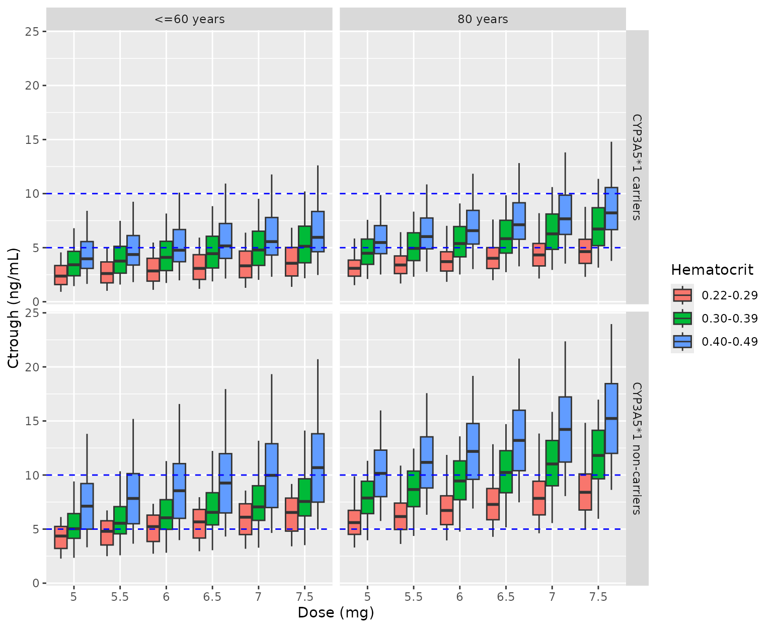
Replicates Figure 3 of Fernandez-Alarcon 2024: simulated day-5 Ctrough by once-daily dose, CYP3A5 genotype, age and hematocrit band. Boxes are the 25th-75th percentiles, whiskers the 5th-95th; dashed lines mark the 5-10 ng/mL target range.
Replicate Figure 4 (day-5 AUC24)
ggplot(box_stats(by_dose, "AUC24"), aes(factor(dose), fill = hct_band)) +
  geom_boxplot(
    aes(ymin = ymin, lower = lower, middle = middle, upper = upper, ymax = ymax),
    stat = "identity", position = position_dodge(width = 0.85), width = 0.8
  ) +
  facet_grid(genotype ~ age_group) +
  labs(x = "Dose (mg)", y = "AUC24 (ng*h/mL)", fill = "Hematocrit")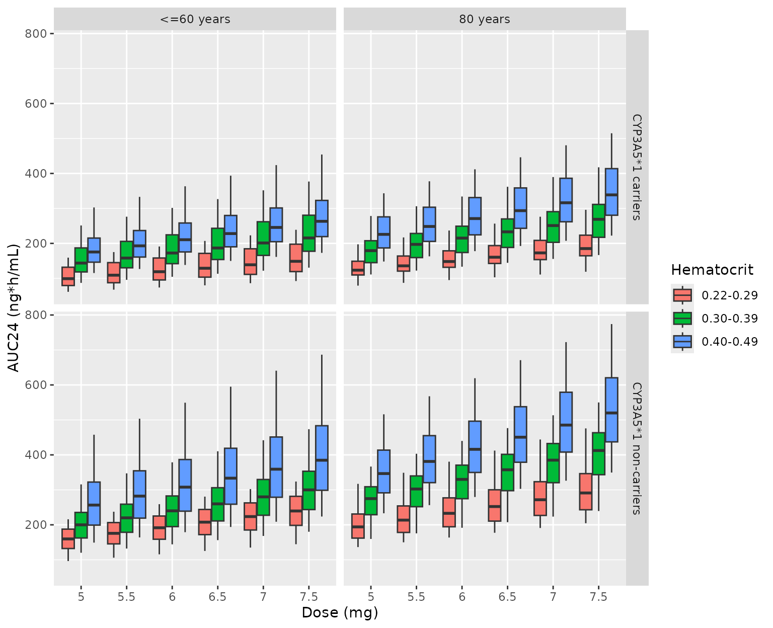
Replicates Figure 4 of Fernandez-Alarcon 2024: simulated day-5 AUC24 by once-daily dose, CYP3A5 genotype, age and hematocrit band. Boxes are the 25th-75th percentiles, whiskers the 5th-95th.
Comparison against the published simulations
The paper prints no exposure table for its simulations, so the reference values below are the medians of the 40-49% hematocrit boxes at 5 mg, digitised by the maintainers from Figures 3 and 4 (reading precision about +/-5%).
published <- tibble::tribble(
  ~arm_label,                          ~auclast, ~cmin,
  "CYP3A5*1 carriers, <=60 years",     185,      4.5,
  "CYP3A5*1 carriers, 80 years",       215,      5.5,
  "CYP3A5*1 non-carriers, <=60 years", 270,      8.0,
  "CYP3A5*1 non-carriers, 80 years",   355,      10.5
)

high_hct_arms <- arms |>
  filter(hct_band == "0.40-0.49") |>
  mutate(arm_label = paste(genotype, age_group, sep = ", "))

nca_high <- as.data.frame(nca_res$result) |>
  dplyr::filter(arm %in% high_hct_arms$arm) |>
  dplyr::left_join(high_hct_arms |> dplyr::select(arm, arm_label), by = "arm") |>
  dplyr::select(arm_label, PPTESTCD, PPORRES)

cmp <- nlmixr2lib::ncaComparisonTable(
  simulated = nca_high,
  reference = published,
  by = "arm_label",
  params = c("auclast", "cmin"),
  units = c(auclast = "ng*h/mL", cmin = "ng/mL"),
  tolerance_pct = 20
)
knitr::kable(
  dplyr::rename(cmp, "Simulated arm" = arm_label),
  caption = paste(
    "Simulated day-5 exposure at 5 mg once daily, hematocrit 40-49%",
    "(median of 100 virtual subjects per arm) versus medians digitised from",
    "Figures 3 and 4 of Fernandez-Alarcon 2024. * differs from reference by >20%."
  )
)| NCA parameter | Simulated arm | Reference | Simulated | % diff |
|---|---|---|---|---|
| Cmin (ng/mL) | CYP3A5*1 carriers, <=60 years | 4.5 | 3.97 | -11.8% |
| Cmin (ng/mL) | CYP3A5*1 carriers, 80 years | 5.5 | 5.48 | -0.4% |
| Cmin (ng/mL) | CYP3A5*1 non-carriers, <=60 years | 8 | 7.12 | -11.0% |
| Cmin (ng/mL) | CYP3A5*1 non-carriers, 80 years | 10.5 | 10.2 | -3.3% |
| AUClast (ng*h/mL) | CYP3A5*1 carriers, <=60 years | 185 | 175 | -5.2% |
| AUClast (ng*h/mL) | CYP3A5*1 carriers, 80 years | 215 | 226 | +5.0% |
| AUClast (ng*h/mL) | CYP3A5*1 non-carriers, <=60 years | 270 | 256 | -5.0% |
| AUClast (ng*h/mL) | CYP3A5*1 non-carriers, 80 years | 355 | 347 | -2.4% |
sim_med <- nca_ind |>
  filter(hct_band == "0.40-0.49") |>
  mutate(arm_label = paste(genotype, age_group, sep = ", ")) |>
  group_by(arm_label) |>
  summarise(auc = median(auclast), ctr = median(cmin), .groups = "drop") |>
  left_join(published, by = "arm_label")
stopifnot(
  # The age effect is the structurally distinctive part of this model: as
  # printed, CL/F drops by 0.0562 * AGE (not 0.0562 * (AGE - 60)) above 60 y,
  # so 80-year-old non-carriers have ~34% higher exposure than younger ones.
  # A mis-encoded age term moves these medians by well over 15%.
  all(abs(sim_med$auc / sim_med$auclast - 1) < 0.15),
  all(abs(sim_med$ctr / sim_med$cmin - 1) < 0.25)
)
Closed-form check of the clearance equation
At steady state AUC_tau = F * Dose / (CL/F) for a linear
model; with the hematocrit standardization the observable whole-blood
AUC is multiplied by HCT / 45. A long typical-value
simulation is compared with that closed form, and the closed form is
compared with the dose-normalised day-5 AUC24 observed in the CYP3A5
genotype groups (Table 3), evaluated at the day-5 median hematocrit of
29.7% (Table 2) and an age of 60 years or younger.
cl_typ <- function(cyp, age, wt = 70) {
  (26.5 * 0.666^(1 - cyp) - 0.0562 * age * (age > 60)) * (wt / 70)^0.75
}
ss_ev <- tidyr::expand_grid(CYP3A5_EXPR = c(1, 0), AGE = c(50, 80)) |>
  mutate(id = row_number(), WT = 70, HCT = 45)
ss_events <- bind_rows(
  ss_ev |> tidyr::expand_grid(time = 24 * 0:29) |>
    mutate(amt = 1, evid = 1L, cmt = "depot"),
  ss_ev |> tidyr::expand_grid(time = seq(24 * 29, 24 * 30, by = 0.05)) |>
    mutate(amt = NA_real_, evid = 0L, cmt = "central")
) |>
  arrange(id, time, desc(evid))
ss_sim <- rxode2::rxSolve(mod_typical, events = ss_events) |>
  as.data.frame()
#> ℹ omega/sigma items treated as zero: 'etalcl', 'etalvc'
#> Warning: multi-subject simulation without without 'omega'
ss_auc <- ss_sim |>
  group_by(id) |>
  summarise(auc_sim = sum(diff(time) * (head(Cc, -1) + tail(Cc, -1)) / 2)) |>
  left_join(ss_ev, by = "id") |>
  mutate(auc_closed = 1000 / cl_typ(CYP3A5_EXPR, AGE))
# Same parameters on both sides: the difference is accumulation (30 doses) and
# trapezoidal error only.
stopifnot(all(abs(ss_auc$auc_sim / ss_auc$auc_closed - 1) < 0.01))

tibble::tibble(
  genotype = c("CYP3A5*1 carriers", "CYP3A5*1 non-carriers"),
  cl = c(cl_typ(1, 50), cl_typ(0, 50)),
  observed = c(22.43, 38.21)
) |>
  mutate(
    predicted = 1000 / cl * 29.7 / 45,
    pct = round(100 * (predicted / observed - 1), 1)
  ) |>
  dplyr::rename(
    "CYP3A5 group" = genotype,
    "Typical CL/F (L/h)" = cl,
    "Observed AUC24/D, Table 3 (ng*h/mL per mg)" = observed,
    "Predicted SS AUC24/D at HCT 29.7% (ng*h/mL per mg)" = predicted,
    "% difference" = pct
  ) |>
knitr::kable(digits = 1)| CYP3A5 group | Typical CL/F (L/h) | Observed AUC24/D, Table 3 (ng*h/mL per mg) | Predicted SS AUC24/D at HCT 29.7% (ng*h/mL per mg) | % difference |
|---|---|---|---|---|
| CYP3A5*1 carriers | 26.5 | 22.4 | 24.9 | 11.0 |
| CYP3A5*1 non-carriers | 17.6 | 38.2 | 37.4 | -2.1 |
The non-carrier prediction is within a few percent of the observed geometric mean. The carrier prediction is about 11% higher, within the Table 3 95% CI (15.6-32.2 ng*h/mL per mg), and the observed values come from day 5, before steady state, in patients of all ages and hematocrits.
Assumptions and deviations
- Hematocrit standardization. The paper states that whole-blood concentrations were standardized to a hematocrit of 45% (Methods 2.6.2, following Storset 2014) and that hematocrit entered through the residual-error block, but it does not print the formula. The packaged model uses the linear form of the cited method, observed whole-blood concentration = standardized concentration x HCT / 45 (HCT in percent). The authors’ own simulations support it: in Figure 4 the median AUC24 ratios between the hematocrit bands match the ratios of the band midpoints (about 0.57 and 0.78 of the 40-49% band).
-
Age effect. Table 4 and Equation 3 both print the
age term as
theta3 * AGE * agecat, the whole age multiplied by the above-60 indicator, nottheta3 * (AGE - 60) * agecat. This makes CL/F drop by about 3.4 L/h in a step at 60 years. The equation is packaged as printed; the Figure 3 and 4 simulations agree with it (80-year-old non-carriers about 30% above younger ones), whereas the(AGE - 60)reading would give only about 7%. -
Where body weight enters. The allometric factor
multiplies the whole bracket
(theta1 * theta2 - theta3 * AGE * agecat), as Table 4 prints it. -
Between-patient variability. Table 4 gives the
variances as CV%; they are converted with
omega^2 = log(1 + CV^2). Inter-occasion variability on CL/F was tested but is not in the final model (Table 4) and is not packaged. - Simulation design. Day 5 is taken as the fifth once-daily dosing interval and Ctrough as the pre-dose trough of that dose. The paper does not say whether its simulated trough is pre-dose or 24 h after the day-5 dose, nor whether residual error was added; the comparison uses medians, which residual error does not shift. The reference values are digitised from the figures, not tabulated in the paper.
-
No non-paper-derived parameter values. Every
ini()value comes from Table 4.