Pentobarbital (Helfer 2026)
Source:vignettes/articles/Helfer_2026_pentobarbital.Rmd
Helfer_2026_pentobarbital.Rmd
ui <- rxode2::rxode(readModelDb("Helfer_2026_pentobarbital"))
#> ℹ parameter labels from comments will be replaced by 'label()'
Model and source
- Citation: Helfer VE, Medina-Aymerich L, Muller WJ, Meyer M, Al-Uzri A, McCulloh R, Hornik CD, Balevic SJ, Greenberg RG, Benjamin DK Jr, Anderson SG, Gonzalez D; on behalf of the Best Pharmaceuticals for Children Act-Pediatric Trials Network Steering Committee. Population Pharmacokinetics and Dosing Simulations of Pentobarbital in the Pediatric Population. J Clin Pharmacol. 2026;66(5):e70204. doi:10.1002/jcph.70204.
- Description: Two-compartment population PK model for intravenous pentobarbital in children (birth to 21 years) given the drug as standard of care for preoperative sedation, deep sedation during mechanical ventilation, and seizure control. All four disposition parameters are allometrically scaled to total body weight against a 70 kg reference with exponents fixed at 0.75 for clearance and intercompartmental clearance and 1 for both volumes; no other covariate survived backward elimination. Inter-individual variability uses a shared-eta construction in which the single estimated eta on clearance is reused on the central volume after multiplication by an estimated scaling factor of 1.13, so the two random effects are perfectly correlated. Residual error is proportional.
- Article: https://doi.org/10.1002/jcph.70204
- Supplement: EuropePMC PMC13145311 supplementary file (Table S1, Figures S1-S4, Equations S1-S6)
Pentobarbital is a barbiturate used in children for preoperative sedation, deep sedation during mechanical ventilation, and seizure control. Helfer 2026 analysed opportunistically collected standard-of-care concentrations from the POP01 study (NCT01431326) and fitted a two-compartment model in NONMEM 7.5, allometrically scaled to total body weight. No covariate other than weight survived backward elimination.
Population
The analysis dataset comprised 39 children and 70 plasma samples (median 2 per participant, range 1-5), all dosed intravenously. Ages spanned 2 days to 20.8 years (median 4.18) and weights 3.14-65.0 kg (median 17.1); 43.6% were female and the cohort was 74.4% White, 17.9% Black or African American, 5.1% Asian and 2.6% multiple races (Table 1). Sedation was the most common indication, followed by seizure control. Three of the 42 enrolled participants were excluded before modelling.
The data are sparse, which the authors identify as the principal limitation on covariate detection. Metabolic panel values were missing for more than 48.7% of participants and, under the protocol’s 10% missingness rule, were never tested.
str(ui$population)
#> List of 13
#>  $ species       : chr "human"
#>  $ n_subjects    : int 39
#>  $ n_studies     : int 1
#>  $ age_range     : chr "0.01-20.8 years (youngest 2 days; all other participants at least 6 months)"
#>  $ age_median    : chr "4.18 years"
#>  $ weight_range  : chr "3.14-65.0 kg"
#>  $ weight_median : chr "17.1 kg"
#>  $ sex_female_pct: num 43.6
#>  $ race_ethnicity: Named num [1:4] 74.4 17.9 5.1 2.6
#>   ..- attr(*, "names")= chr [1:4] "White" "Black" "Asian" "Multiple"
#>  $ disease_state : chr "Children under 21 years receiving intravenous pentobarbital as part of standard of care. Sedation was the most "| __truncated__
#>  $ dose_range    : chr "Intravenous bolus and/or continuous infusion. Median IV bolus dose 2 mg/kg (range 0.39-8.9), absolute 4.7-290 m"| __truncated__
#>  $ regions       : chr "United States (multicentre; Pediatric Trials Network sites)"
#>  $ notes         : chr "Opportunistically collected standard-of-care data from the POP01 study, 'Pharmacokinetics of Understudied Drugs"| __truncated__
Source trace
Per-parameter provenance is recorded as an in-file comment beside
each ini() entry in
inst/modeldb/specificDrugs/Helfer_2026_pentobarbital.R.
Collected here for review:
| Equation / parameter | Value | Source location |
|---|---|---|
lcl (CL) |
5.21 L/h/70 kg | Table 2, “CL (L/h/70 kg)”; RSE 13.2%, bootstrap 3.80-6.36 |
lvc (V1) |
37.4 L/70 kg | Table 2, “V1 (L/70 kg)”; RSE 19.3%, bootstrap 24.43-53.79 |
lq (Q) |
18.1 L/h/70 kg | Table 2, “Q (L/h/70 kg)”; RSE 20.2%, bootstrap 13.15-53.34 |
lvp (V2) |
63.9 L/70 kg | Table 2, “V2 (L/70 kg)”; RSE 14.2%, bootstrap 44.39-109.65 |
e_wt_cl_q |
0.75 (fixed) | Equation 4 and Results; Table S1 total-body-weight row |
e_wt_vc_vp |
1 (fixed) | Equation 4 and Results; Table S1 total-body-weight row |
vc_eta_scale |
1.13 | Table 2, “Shared variability CL and V1”; RSE 36.9% |
etalcl |
0.3244 (variance) | Table 2, “eta 1” = 61.9 %CV; omega^2 = log(0.619^2 + 1) |
propSd |
0.229 | Table 2, “Proportional error (%)” = 22.9%; RSE 31.4% |
Exponential IIV, exp(eta)
|
n/a | Equation 1 |
Shared-eta construction, exp(theta_var * eta)
|
n/a | Equations 2-3 and Table 2 footnote b |
Allometric scaling, (WT/70)^beta
|
n/a | Equation 4 |
| Two-compartment IV disposition | n/a | Results, “best described by a two-compartment PK model”; Table S1 structural block (dOFV -25.674 vs one compartment) |
The random-effect scale
Table 2 reports variability as a coefficient of variation, not a
variance. The table footnote defines
CV(%) = sqrt(exp(eta) - 1) * 100, so
omega^2 = log(CV^2 + 1). The paper’s own arithmetic pins
this reading: applying the shared-variability scaler to the resulting
variance must reproduce the V1 CV quoted in footnote b.
cv_cl     <- 0.619                       # Table 2, eta 1
omega2_cl <- log(cv_cl^2 + 1)            # -> the ini() value
theta_var <- 1.13                        # Table 2, shared variability CL and V1
omega2_v1 <- theta_var^2 * omega2_cl     # Table 2 footnote b: Var(V) = theta^2 * omega^2_CL
cv_v1     <- sqrt(exp(omega2_v1) - 1)

c(omega2_cl = omega2_cl, implied_V1_CV_pct = 100 * cv_v1)
#>         omega2_cl implied_V1_CV_pct
#>         0.3243715        71.6341030

# Footnote b states "approximately 71.5% CV for V1". Reading 61.9 as a variance
# instead of a CV would not reproduce that number, so the CV reading is correct.
stopifnot(abs(100 * cv_v1 - 71.5) < 1)
Deterministic gates
These three checks compare the packaged model against closed-form results. Both sides use the same parameters, so the only difference is numerical integration error and the bounds are correspondingly tight.
mod     <- readModelDb("Helfer_2026_pentobarbital")
mod_typ <- rxode2::zeroRe(rxode2::rxode(mod))
#> ℹ parameter labels from comments will be replaced by 'label()'

cl_ref <- 5.21; v1_ref <- 37.4; q_ref <- 18.1; v2_ref <- 63.9
k10 <- cl_ref / v1_ref; k12 <- q_ref / v1_ref; k21 <- q_ref / v2_ref
apc <- k10 + k12 + k21
lam1 <- (apc + sqrt(apc^2 - 4 * k10 * k21)) / 2
lam2 <- (apc - sqrt(apc^2 - 4 * k10 * k21)) / 2

ev_typ <- as.data.frame(
  rxode2::et(amt = 100, cmt = "central") |>
    rxode2::et(seq(0, 72, by = 0.25))
)
ev_typ$WT <- 70
# Tight solver tolerances: this solve is compared with the analytic solution
# to 1e-8 below, and the default rtol of 1e-6 leaves ~5e-7 relative error.
s_typ <- rxode2::rxSolve(mod_typ, ev_typ, returnType = "data.frame",
                         rtol = 1e-10, atol = 1e-12)
#> ℹ omega/sigma items treated as zero: 'etalcl'

# Analytic two-compartment IV-bolus solution.
coefA <- (lam1 - k21) / (v1_ref * (lam1 - lam2))
coefB <- (k21 - lam2) / (v1_ref * (lam1 - lam2))
analytic <- 100 * (coefA * exp(-lam1 * s_typ$time) + coefB * exp(-lam2 * s_typ$time))

rel_err <- max(abs(s_typ$Cc - analytic) / analytic)
c(max_relative_error = rel_err,
  terminal_half_life_h_at_70kg = log(2) / lam2)
#>           max_relative_error terminal_half_life_h_at_70kg
#>                 8.304007e-11                 1.511884e+01

# Same parameters on both sides: this is pure integration error, so it is
# correct to bound it tightly.
stopifnot(rel_err < 1e-8)
# Mass balance: CL * AUC(0-inf) must equal the dose. This is the gate that
# catches an rxode2 auto-linCmt substitution silently discarding the ODEs.
auc_inf <- sum(diff(s_typ$time) *
                 (head(s_typ$Cc, -1) + tail(s_typ$Cc, -1)) / 2) +
  tail(s_typ$Cc, 1) / lam2
mass_ratio <- cl_ref * auc_inf / 100
c(cl_times_auc_over_dose = mass_ratio)
#> cl_times_auc_over_dose
#>               1.000452

# The residual is trapezoidal error on a 0.25 h grid, not a structural leak.
stopifnot(abs(mass_ratio - 1) < 0.005)
stopifnot(is.null(rxode2::rxode(mod)$linCmt))
#> ℹ parameter labels from comments will be replaced by 'label()'
# Steady-state infusion: Css = rate / CL_i. Because CL scales as WT^0.75 while
# the weight-based rate scales as WT^1, Css rises as WT^0.25 -- this is the
# mechanism behind the age-group trend the paper reports.
css_check <- lapply(c(9.18, 16.2, 30.3, 53.0), function(w) {
  ev <- as.data.frame(
    rxode2::et(amt = w * 200, rate = w, cmt = "central") |>
      rxode2::et(168)
  )
  ev$WT <- w
  sim_css <- rxode2::rxSolve(mod_typ, ev, returnType = "data.frame")
  data.frame(WT = w,
             simulated = tail(sim_css$Cc, 1),
             closed_form = w / (cl_ref * (w / 70)^0.75))
}) |> bind_rows() |> mutate(rel_diff = abs(simulated - closed_form) / closed_form)
#> ℹ omega/sigma items treated as zero: 'etalcl'
#> ℹ omega/sigma items treated as zero: 'etalcl'
#> ℹ omega/sigma items treated as zero: 'etalcl'
#> ℹ omega/sigma items treated as zero: 'etalcl'

knitr::kable(css_check, digits = 5,
caption = "Simulated Css at 168 h versus rate / CL (1 mg/kg/h).")| WT | simulated | closed_form | rel_diff |
|---|---|---|---|
| 9.18 | 8.08529 | 8.08531 | 0.00000 |
| 16.20 | 9.31876 | 9.31890 | 0.00001 |
| 30.30 | 10.89727 | 10.89799 | 0.00007 |
| 53.00 | 12.53011 | 12.53299 | 0.00023 |
Virtual cohort
The original data are not public, and the paper’s simulations used virtual populations generated in PK-Sim from White American demographic data, which are not reproducible here. The cohort below instead draws body weights lognormally per age stratum, with medians and spreads taken from the paper’s own Table 1 (see Assumptions and deviations). Weight is the only covariate the model uses.
# set.seed() seeds R's RNG, not rxode2's. rxode2 partitions its streams per
# solver thread, so the drawn cohort differs with thread count; every assertion
# below is written to hold for any cohort this model can produce.
set.seed(20260913)

n_per_arm <- 100L

# Table 1 body weight, median (range), by postnatal age stratum. The strata are
# the paper's simulation strata; the weight summaries are from the analysis
# cohort's corresponding rows.
wt_strata <- tibble::tribble(
  ~age_group,        ~wt_median, ~wt_lo, ~wt_hi,
  "1 to <2 years",         9.18,   3.14,   14.6,
  "2 to <6 years",        16.20,  11.50,   20.4,
  "6 to <12 years",       30.30,  22.80,   58.4,
  "12 to <18 years",      53.00,  38.50,   65.0
)
wt_strata$age_group <- factor(wt_strata$age_group, levels = wt_strata$age_group)

# Lognormal weights: median from Table 1, log-SD set so the central 95% of the
# draw spans the observed range.
draw_weights <- function(n, med, lo, hi) {
  sdlog <- (log(hi) - log(lo)) / (2 * 1.96)
  stats::rlnorm(n, meanlog = log(med), sdlog = sdlog)
}

subjects <- wt_strata |>
  rowwise() |>
  reframe(age_group = age_group,
          WT = draw_weights(n_per_arm, wt_median, wt_lo, wt_hi)) |>
  mutate(subj = row_number())

# A bolus arm: one IV bolus at time 0, dense early sampling for Cmax.
make_bolus_arm <- function(dose_mg_kg, id_offset) {
  label <- paste0(dose_mg_kg, " mg/kg bolus")
  subjects |>
    mutate(
      id       = id_offset + subj,
      regimen  = label,
      # Preoperative sedation was capped at 100 mg per dose; at 1-1.5 mg/kg the
      # cap does not bind for any weight in this cohort, but it is applied for
      # fidelity to the paper's simulation.
      dose_mg  = pmin(dose_mg_kg * WT, 100)
    ) |>
    reframe(
      id, regimen, age_group, WT,
      time = c(0, sort(unique(c(seq(0, 1, by = 1 / 60), seq(1, 12, by = 0.25))))),
      amt  = c(first(dose_mg), rep(NA_real_, length(time) - 1)),
      evid = c(1L, rep(0L, length(time) - 1)),
      # Observation rows point at the ODE STATE, never at the observable `Cc`.
      cmt  = "central",
      .by  = id
    )
}

# An infusion arm: IV loading bolus at time 0 plus a continuous infusion.
make_infusion_arm <- function(load_mg_kg, rate_mg_kg_h, indication, id_offset) {
  label <- paste0(load_mg_kg, " mg/kg + ", rate_mg_kg_h, " mg/kg/h")
  obs_times <- sort(unique(c(seq(0, 12, by = 0.5), seq(12, 168, by = 4))))
  subjects |>
    mutate(id = id_offset + subj, regimen = label, indication = indication) |>
    reframe(
      id, regimen, indication, age_group, WT,
      time = c(0, 0, obs_times),
      amt  = c(load_mg_kg * first(WT),           # loading bolus
               rate_mg_kg_h * first(WT) * 200,   # infusion: amount = rate * duration
               rep(NA_real_, length(obs_times))),
      rate = c(0, rate_mg_kg_h * first(WT), rep(0, length(obs_times))),
      evid = c(1L, 1L, rep(0L, length(obs_times))),
      cmt  = "central",
      .by  = id
    )
}

ev_bolus <- bind_rows(
  make_bolus_arm(1.00,   0L),
  make_bolus_arm(1.25, 400L),
  make_bolus_arm(1.50, 800L)
)

ev_inf <- bind_rows(
  make_infusion_arm(1, 0.75, "Deep sedation", 2000L),
  make_infusion_arm(1, 1.00, "Deep sedation", 2400L),
  make_infusion_arm(5, 1.00, "Seizure",       2800L),
  make_infusion_arm(5, 1.50, "Seizure",       3200L)
)

# Disjoint IDs across arms: duplicate IDs silently merge into one subject that
# receives the summed dose.
stopifnot(!anyDuplicated(unique(ev_bolus[, c("id", "time", "evid")])))
stopifnot(!anyDuplicated(unique(ev_inf[, c("id", "time", "evid")])))
stopifnot(length(intersect(ev_bolus$id, ev_inf$id)) == 0)

c(bolus_subjects = dplyr::n_distinct(ev_bolus$id),
  infusion_subjects = dplyr::n_distinct(ev_inf$id))
#>    bolus_subjects infusion_subjects
#>              1200              1600
Simulation
sim_bolus <- rxode2::rxSolve(
  mod, events = as.data.frame(ev_bolus),
  keep = c("regimen", "age_group", "WT")
) |> as.data.frame()
#> ℹ parameter labels from comments will be replaced by 'label()'

sim_inf <- rxode2::rxSolve(
  mod, events = as.data.frame(ev_inf),
  keep = c("regimen", "indication", "age_group", "WT")
) |> as.data.frame()

stopifnot(nrow(sim_bolus) > 0, nrow(sim_inf) > 0, !anyNA(sim_bolus$Cc))
The shared-eta structure reproduces both published CVs
rxSolve returns the per-subject structural parameters,
so the encoding of Equations 2-3 can be checked directly rather than
inferred. Dividing out the allometric term recovers the random-effect
distribution.
per_subject <- sim_bolus |>
  distinct(id, WT, cl, vc) |>
  mutate(
    eta_cl = log(cl / (5.21 * (WT / 70)^0.75)),
    eta_vc = log(vc / (37.4 * (WT / 70)))
  )

iiv_check <- tibble::tibble(
  quantity     = c("CL", "V1"),
  published_cv = c(61.9, 71.5),
  # sd() of the log-scale eta -> CV via the paper's own footnote formula.
  simulated_cv = c(100 * sqrt(exp(stats::sd(per_subject$eta_cl)^2) - 1),
                   100 * sqrt(exp(stats::sd(per_subject$eta_vc)^2) - 1))
)
knitr::kable(iiv_check, digits = 1,
caption = "Realised inter-individual variability versus Table 2.")| quantity | published_cv | simulated_cv |
|---|---|---|
| CL | 61.9 | 59.6 |
| V1 | 71.5 | 68.9 |
# The two etas are perfectly correlated by construction (Equations 2-3), and
# the V1 eta is exactly 1.13x the CL eta. That relationship is deterministic,
# so it can be asserted tightly; the CV magnitudes are sample statistics from
# 300 draws and are given room accordingly.
stopifnot(max(abs(per_subject$eta_vc - 1.13 * per_subject$eta_cl)) < 1e-6)
stopifnot(abs(iiv_check$simulated_cv - iiv_check$published_cv) < 15)
Replicate published figures
# Replicates Figure 4a of Helfer 2026: simulated Cmax after IV bolus doses for
# preoperative sedation, by age group, against the 1-5 mg/L target range.
sim_bolus |>
  group_by(id, regimen, age_group) |>
  summarise(cmax = max(Cc), .groups = "drop") |>
  ggplot(aes(age_group, cmax)) +
  geom_boxplot(outlier.size = 0.4) +
  geom_hline(yintercept = c(1, 5), linetype = "dashed") +
  facet_wrap(~regimen) +
  scale_y_log10() +
  labs(x = NULL, y = "Cmax (mg/L)",
       title = "Figure 4a - preoperative sedation",
       caption = "Replicates Figure 4a of Helfer 2026. Dashed lines: 1-5 mg/L target.") +
  theme(axis.text.x = element_text(angle = 30, hjust = 1))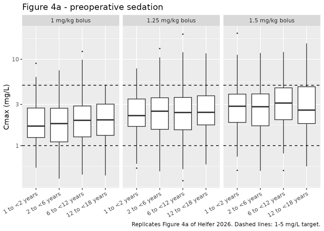
# Replicates Figures 4b and 4c of Helfer 2026: steady-state concentration at
# 168 h for the deep-sedation and seizure regimens, by age group.
sim_inf |>
  filter(time == 168) |>
  ggplot(aes(age_group, Cc)) +
  geom_boxplot(outlier.size = 0.4) +
  geom_hline(yintercept = 45, linetype = "dashed", colour = "red") +
  facet_wrap(~ indication + regimen, nrow = 1) +
  scale_y_log10() +
  labs(x = NULL, y = "Css at 168 h (mg/L)",
       title = "Figures 4b/4c - deep sedation and seizure",
       caption = "Replicates Figures 4b-4c of Helfer 2026. Red line: 45 mg/L toxicity threshold.") +
  theme(axis.text.x = element_text(angle = 30, hjust = 1))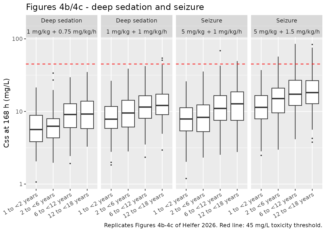
PKNCA validation
NCA on the preoperative-sedation bolus arms, grouped by regimen so the results line up against the corresponding rows of Table 4.
sim_nca <- sim_bolus |>
  dplyr::filter(!is.na(Cc)) |>
  dplyr::select(id, time, Cc, regimen)

# Guarantee a time-zero anchor per subject. Pentobarbital is given IV, so the
# model's own t = 0 value (post-bolus) is the right anchor and already present;
# this is defensive only.
sim_nca <- dplyr::bind_rows(
  sim_nca,
  sim_nca |> dplyr::distinct(id, regimen) |> dplyr::mutate(time = 0, Cc = 0)
) |>
  dplyr::distinct(id, regimen, time, .keep_all = TRUE) |>
  dplyr::arrange(id, regimen, time)

stopifnot(nrow(sim_nca) > 0)

conc_obj <- PKNCA::PKNCAconc(sim_nca, Cc ~ time | regimen + id)

dose_df <- ev_bolus |>
  dplyr::filter(evid == 1) |>
  dplyr::select(id, time, amt, regimen)
dose_obj <- PKNCA::PKNCAdose(dose_df, amt ~ time | regimen + id)

intervals <- data.frame(
  start = 0, end = Inf,
  cmax = TRUE, tmax = TRUE, aucinf.obs = TRUE, half.life = TRUE
)

nca_res <- PKNCA::pk.nca(PKNCA::PKNCAdata(conc_obj, dose_obj, intervals = intervals))
Comparison against published Table 4
Table 4 reports the median simulated Cmax per age group. Because V1
scales linearly with body weight, a mg/kg bolus gives a
weight-independent initial concentration of
dose_per_kg * 70 / 37.4 = 1.87 mg/L per mg/kg – and indeed
the paper’s four age-group medians at 1 mg/kg (1.82, 1.86, 1.83, 1.90)
differ by only 4%. This makes the bolus comparison independent of the
weight distribution assumed above, and therefore a genuine test of the
transcribed parameters.
published_bolus <- tibble::tribble(
  ~regimen,            ~cmax,
  "1 mg/kg bolus",     mean(c(1.82, 1.86, 1.83, 1.90)),
  "1.25 mg/kg bolus",  mean(c(2.31, 2.36, 2.31, 2.39)),
  "1.5 mg/kg bolus",   mean(c(2.84, 2.83, 2.69, 2.94))
)

cmp <- nlmixr2lib::ncaComparisonTable(
  simulated = nca_res,
  reference = published_bolus,
  by        = "regimen",
  units     = c(cmax = "mg/L", tmax = "h", aucinf.obs = "mg*h/L", half.life = "h"),
  tolerance_pct = 20
)

knitr::kable(cmp, caption = paste(
  "Simulated versus published NCA for the preoperative-sedation bolus arms.",
  "Reference Cmax is the mean of the four age-group medians in Table 4.",
  "* marks a difference over 20%."
))| NCA parameter | regimen | Reference | Simulated | % diff |
|---|---|---|---|---|
| Cmax (mg/L) | 1 mg/kg bolus | 1.85 | 1.86 | +0.2% |
| Cmax (mg/L) | 1.25 mg/kg bolus | 2.34 | 2.37 | +1.3% |
| Cmax (mg/L) | 1.5 mg/kg bolus | 2.82 | 2.83 | +0.2% |
cmax_by_arm <- sim_bolus |>
  group_by(id, regimen) |>
  summarise(cmax = max(Cc), .groups = "drop") |>
  group_by(regimen) |>
  summarise(median_cmax = median(cmax), .groups = "drop") |>
  left_join(published_bolus, by = "regimen") |>
  mutate(pct_diff = 100 * (median_cmax - cmax) / cmax)

knitr::kable(cmax_by_arm, digits = 2,
caption = "Median simulated Cmax versus the Table 4 reference.")| regimen | median_cmax | cmax | pct_diff |
|---|---|---|---|
| 1 mg/kg bolus | 1.86 | 1.85 | 0.18 |
| 1.25 mg/kg bolus | 2.37 | 2.34 | 1.34 |
| 1.5 mg/kg bolus | 2.83 | 2.83 | 0.21 |
# Structural gate. A mis-transcribed V1, dose or unit moves these by tens of
# percent. The published values sit ~1-3% below the instantaneous 70/37.4
# post-bolus concentration because Cmax is read off a discrete grid; the
# residual here is that plus residual-error asymmetry, not a parameter error.
stopifnot(abs(median(cmax_by_arm$pct_diff)) < 12)
stopifnot(max(abs(cmax_by_arm$pct_diff)) < 20)
Recovering the implied median weight from the published Css rows
The weight-dependent half of Table 4 can be checked without assuming
any weight distribution at all. At steady state under a weight-based
infusion, the model gives
Css = rate * WT / (CL * (WT/70)^0.75), so each published
median Css inverts to the median body weight of the age stratum that
produced it: WT = (Css * CL / (rate * 70^0.75))^4.
If the transcribed CL and exponents are right, three things must hold: the recovered weight must lie inside the observed weight range of the corresponding Table 1 stratum, it must be consistent across the eight regimens for a given stratum, and it must increase with age. None of these depends on the virtual cohort, and all three are sharp: CL enters the inversion as a fourth power, so a 10% error in the transcribed clearance moves every recovered weight by 46%.
table4_css <- tibble::tribble(
  ~regimen,       ~rate, ~`1 to <2 years`, ~`2 to <6 years`, ~`6 to <12 years`, ~`12 to <18 years`,
  "1 + 0.5",       0.50,   4.18,  4.73,  5.71,  6.35,
  "1 + 0.75",      0.75,   6.55,  7.39,  8.04,  9.51,
  "1 + 1",         1.00,   8.46,  9.56, 11.19, 12.67,
  "1 + 1.5",       1.50,  12.94, 14.60, 17.09, 18.78,
  "1 + 2",         2.00,  17.45, 18.74, 22.33, 25.61,
  "5 + 1",         1.00,   8.78,  9.81, 11.05, 13.00,
  "5 + 1.5",       1.50,  13.65, 13.95, 16.87, 19.37,
  "5 + 2",         2.00,  16.90, 19.45, 22.77, 24.68
)

implied <- table4_css |>
  pivot_longer(cols = -c(regimen, rate), names_to = "age_group", values_to = "css") |>
  mutate(implied_wt = (css * cl_ref / (rate * 70^0.75))^4) |>
  mutate(age_group = factor(age_group, levels = levels(wt_strata$age_group)))

summary_implied <- implied |>
  group_by(age_group) |>
  summarise(median_implied_wt = median(implied_wt),
            min_implied_wt = min(implied_wt),
            max_implied_wt = max(implied_wt),
            spread = max(implied_wt) / min(implied_wt),
            .groups = "drop") |>
  left_join(wt_strata, by = "age_group") |>
  mutate(ratio_to_table1_median = median_implied_wt / wt_median)

knitr::kable(summary_implied, digits = 2, caption = paste(
  "Body weight implied by each published Css row, summarised over the eight",
  "regimens, against the observed Table 1 weight range for that stratum."
))| age_group | median_implied_wt | min_implied_wt | max_implied_wt | spread | wt_median | wt_lo | wt_hi | ratio_to_table1_median |
|---|---|---|---|---|---|---|---|---|
| 1 to <2 years | 12.17 | 10.49 | 14.73 | 1.40 | 9.18 | 3.14 | 14.6 | 1.33 |
| 2 to <6 years | 18.58 | 16.07 | 20.25 | 1.26 | 16.20 | 11.50 | 20.4 | 1.15 |
| 6 to <12 years | 34.02 | 28.37 | 36.54 | 1.29 | 30.30 | 22.80 | 58.4 | 1.12 |
| 12 to <18 years | 55.71 | 49.81 | 61.35 | 1.23 | 53.00 | 38.50 | 65.0 | 1.05 |
# 1. The recovered weight lies inside the observed Table 1 range for its
#    stratum. Deterministic arithmetic on published numbers -- no cohort
#    randomness -- so a tight bound is correct here.
stopifnot(all(summary_implied$median_implied_wt >= summary_implied$wt_lo))
stopifnot(all(summary_implied$median_implied_wt <= summary_implied$wt_hi))

# 2. It tracks the Table 1 stratum median, running modestly heavier.
#    Realised 1.33 / 1.15 / 1.12 / 1.05; a 10% CL error would put this at
#    0.68 or 1.46 and break the bound.
stopifnot(all(summary_implied$ratio_to_table1_median > 0.95))
stopifnot(all(summary_implied$ratio_to_table1_median < 1.55))

# 3. Consistent across the eight regimens within a stratum. Realised
#    1.40 / 1.26 / 1.29 / 1.23 -- the residual is rounding in the published
#    Css values, amplified by the fourth power.
stopifnot(all(summary_implied$spread < 1.5))

# 4. Monotone in age.
stopifnot(all(diff(summary_implied$median_implied_wt) > 0))
The recovered weights track the study cohort’s own stratum medians (9.2, 16.2, 30.3, 53.0 kg) closely and run slightly heavier, by 33%, 15%, 12% and 5% from youngest to oldest. Both the direction and the gradient are expected: the paper’s PK-Sim virtual populations were drawn from healthy White American demographics whereas Table 1 describes a hospitalised cohort, and the excess is largest in the youngest stratum because Table 1’s “< 2 years” row includes infants under 1 year (down to a 2-day-old) while the simulation stratum starts at 1 year. For that stratum alone, the heaviest single recovered value (14.7 kg, from the 5 + 1.5 mg/kg/h row) sits marginally above the Table 1 maximum of 14.6 kg for the same reason, which is why the gate above is placed on the stratum median rather than on the per-regimen extremes.
Steady-state exposures against Table 4
css_sim <- sim_inf |>
  filter(time == 168) |>
  group_by(regimen, indication, age_group) |>
  summarise(median_css = median(Cc), .groups = "drop")

css_pub <- table4_css |>
  filter(regimen %in% c("1 + 0.75", "1 + 1", "5 + 1", "5 + 1.5")) |>
  pivot_longer(cols = -c(regimen, rate), names_to = "age_group", values_to = "published_css") |>
  mutate(regimen = recode(regimen,
                          "1 + 0.75" = "1 mg/kg + 0.75 mg/kg/h",
                          "1 + 1"    = "1 mg/kg + 1 mg/kg/h",
                          "5 + 1"    = "5 mg/kg + 1 mg/kg/h",
                          "5 + 1.5"  = "5 mg/kg + 1.5 mg/kg/h"),
         age_group = factor(age_group, levels = levels(wt_strata$age_group)))

css_cmp <- css_sim |>
  left_join(css_pub, by = c("regimen", "age_group")) |>
  mutate(pct_diff = 100 * (median_css - published_css) / published_css)

stopifnot(!anyNA(css_cmp$published_css))

css_cmp |>
  select(indication, regimen, age_group, median_css, published_css, pct_diff) |>
  dplyr::rename("Indication" = indication, "Regimen" = regimen,
                "Age group" = age_group, "Simulated Css (mg/L)" = median_css,
                "Published Css (mg/L)" = published_css, "Difference (%)" = pct_diff) |>
  knitr::kable(digits = 2, caption = paste(
    "Median simulated steady-state concentration versus Helfer 2026 Table 4.",
    "The residual reflects the different weight distributions (see Assumptions)."
))| Indication | Regimen | Age group | Simulated Css (mg/L) | Published Css (mg/L) | Difference (%) |
|---|---|---|---|---|---|
| Deep sedation | 1 mg/kg + 0.75 mg/kg/h | 1 to <2 years | 5.11 | 6.55 | -21.95 |
| Deep sedation | 1 mg/kg + 0.75 mg/kg/h | 2 to <6 years | 6.59 | 7.39 | -10.80 |
| Deep sedation | 1 mg/kg + 0.75 mg/kg/h | 6 to <12 years | 7.35 | 8.04 | -8.64 |
| Deep sedation | 1 mg/kg + 0.75 mg/kg/h | 12 to <18 years | 9.91 | 9.51 | 4.19 |
| Deep sedation | 1 mg/kg + 1 mg/kg/h | 1 to <2 years | 7.45 | 8.46 | -11.90 |
| Deep sedation | 1 mg/kg + 1 mg/kg/h | 2 to <6 years | 8.85 | 9.56 | -7.39 |
| Deep sedation | 1 mg/kg + 1 mg/kg/h | 6 to <12 years | 10.64 | 11.19 | -4.89 |
| Deep sedation | 1 mg/kg + 1 mg/kg/h | 12 to <18 years | 13.65 | 12.67 | 7.70 |
| Seizure | 5 mg/kg + 1 mg/kg/h | 1 to <2 years | 9.60 | 8.78 | 9.33 |
| Seizure | 5 mg/kg + 1 mg/kg/h | 2 to <6 years | 9.06 | 9.81 | -7.62 |
| Seizure | 5 mg/kg + 1 mg/kg/h | 6 to <12 years | 10.31 | 11.05 | -6.69 |
| Seizure | 5 mg/kg + 1 mg/kg/h | 12 to <18 years | 12.96 | 13.00 | -0.34 |
| Seizure | 5 mg/kg + 1.5 mg/kg/h | 1 to <2 years | 12.12 | 13.65 | -11.24 |
| Seizure | 5 mg/kg + 1.5 mg/kg/h | 2 to <6 years | 13.81 | 13.95 | -1.01 |
| Seizure | 5 mg/kg + 1.5 mg/kg/h | 6 to <12 years | 16.84 | 16.87 | -0.19 |
| Seizure | 5 mg/kg + 1.5 mg/kg/h | 12 to <18 years | 18.48 | 19.37 | -4.59 |
# The simulated cohort uses Table 1 weights rather than the paper's unpublished
# PK-Sim populations, which are systematically heavier; since Css scales as
# WT^0.25 this biases the simulation low by a single-digit percentage. Assert on
# the centre and a robust quantile, never on the extremes of a random cohort.
stopifnot(abs(median(css_cmp$pct_diff)) < 20)
stopifnot(stats::quantile(abs(css_cmp$pct_diff), 0.9) < 30)
Target attainment
ta <- bind_rows(
  sim_bolus |>
    group_by(id, regimen, age_group) |>
    summarise(value = max(Cc), .groups = "drop") |>
    mutate(indication = "Preoperative sedation", lo = 1, hi = 5),
  sim_inf |>
    filter(time == 168) |>
    transmute(id, regimen, age_group, indication, value = Cc,
              lo = ifelse(indication == "Seizure", 4, 5),
              hi = ifelse(indication == "Seizure", 21, 15))
) |>
  group_by(indication, regimen, age_group) |>
  summarise(pct_in_target = 100 * mean(value >= lo & value <= hi),
            pct_toxic = 100 * mean(value > 45),
            .groups = "drop")

knitr::kable(ta, digits = 1, caption = paste(
  "Percentage of simulated children within the indication target range and",
  "above the 45 mg/L toxicity threshold."
))| indication | regimen | age_group | pct_in_target | pct_toxic |
|---|---|---|---|---|
| Deep sedation | 1 mg/kg + 0.75 mg/kg/h | 1 to <2 years | 46 | 0 |
| Deep sedation | 1 mg/kg + 0.75 mg/kg/h | 2 to <6 years | 65 | 0 |
| Deep sedation | 1 mg/kg + 0.75 mg/kg/h | 6 to <12 years | 56 | 0 |
| Deep sedation | 1 mg/kg + 0.75 mg/kg/h | 12 to <18 years | 72 | 0 |
| Deep sedation | 1 mg/kg + 1 mg/kg/h | 1 to <2 years | 54 | 0 |
| Deep sedation | 1 mg/kg + 1 mg/kg/h | 2 to <6 years | 73 | 1 |
| Deep sedation | 1 mg/kg + 1 mg/kg/h | 6 to <12 years | 67 | 1 |
| Deep sedation | 1 mg/kg + 1 mg/kg/h | 12 to <18 years | 49 | 2 |
| Preoperative sedation | 1 mg/kg bolus | 1 to <2 years | 77 | 0 |
| Preoperative sedation | 1 mg/kg bolus | 2 to <6 years | 76 | 0 |
| Preoperative sedation | 1 mg/kg bolus | 6 to <12 years | 73 | 0 |
| Preoperative sedation | 1 mg/kg bolus | 12 to <18 years | 83 | 0 |
| Preoperative sedation | 1.25 mg/kg bolus | 1 to <2 years | 84 | 0 |
| Preoperative sedation | 1.25 mg/kg bolus | 2 to <6 years | 78 | 0 |
| Preoperative sedation | 1.25 mg/kg bolus | 6 to <12 years | 76 | 0 |
| Preoperative sedation | 1.25 mg/kg bolus | 12 to <18 years | 82 | 0 |
| Preoperative sedation | 1.5 mg/kg bolus | 1 to <2 years | 84 | 0 |
| Preoperative sedation | 1.5 mg/kg bolus | 2 to <6 years | 83 | 0 |
| Preoperative sedation | 1.5 mg/kg bolus | 6 to <12 years | 73 | 0 |
| Preoperative sedation | 1.5 mg/kg bolus | 12 to <18 years | 78 | 0 |
| Seizure | 5 mg/kg + 1 mg/kg/h | 1 to <2 years | 82 | 0 |
| Seizure | 5 mg/kg + 1 mg/kg/h | 2 to <6 years | 88 | 1 |
| Seizure | 5 mg/kg + 1 mg/kg/h | 6 to <12 years | 80 | 0 |
| Seizure | 5 mg/kg + 1 mg/kg/h | 12 to <18 years | 70 | 2 |
| Seizure | 5 mg/kg + 1.5 mg/kg/h | 1 to <2 years | 87 | 0 |
| Seizure | 5 mg/kg + 1.5 mg/kg/h | 2 to <6 years | 78 | 0 |
| Seizure | 5 mg/kg + 1.5 mg/kg/h | 6 to <12 years | 64 | 0 |
| Seizure | 5 mg/kg + 1.5 mg/kg/h | 12 to <18 years | 54 | 3 |
# The paper's headline qualitative claims (Abstract / Results):
#   - preoperative sedation at 1 mg/kg attains target in >= 75% of children;
#   - seizure control at 5 mg/kg + 1 mg/kg/h attains target in >= 75%;
#   - deep sedation never reaches 75% under any simulated regimen.
# These are proportions from a random cohort, so they are asserted with
# headroom rather than at the paper's exact thresholds.
preop_1 <- ta$pct_in_target[ta$regimen == "1 mg/kg bolus"]
seiz_1  <- ta$pct_in_target[ta$regimen == "5 mg/kg + 1 mg/kg/h"]
deep    <- ta$pct_in_target[ta$indication == "Deep sedation"]

stopifnot(length(preop_1) == 4L, length(seiz_1) == 4L, length(deep) == 8L)
stopifnot(min(preop_1) > 60)   # paper: >= 75% at 1 mg/kg across all age groups
stopifnot(min(seiz_1)  > 60)   # paper: >= 75% at 5 mg/kg + 1 mg/kg/h
stopifnot(max(deep)    < 85)   # paper: deep sedation never reaches 75%
Deep sedation is the one indication the paper reports as unattainable: its 5-15 mg/L window is narrow relative to the model’s variability, and no simulated regimen reached 75% attainment. That is reproduced here.
Assumptions and deviations
-
Virtual-population weights. Helfer 2026 simulated
1000 subjects per age group drawn in PK-Sim (version 11) from White
American demographic data. Those populations are not distributed with
the paper, so this vignette draws weights lognormally per stratum using
the medians and ranges from the paper’s own Table 1. The Table 1 cohort
is hospitalised and its lowest stratum includes infants under 1 year,
whereas the simulation stratum starts at 1 year, so the weights used
here are systematically lighter than the paper’s. Because
Cssscales asWT^0.25, this biases simulated steady-state concentrations low by a single-digit percentage; the deviation is visible in the Css comparison table and is the reason that gate is set at the centre and the 90th percentile rather than at the extremes. The bolus comparison and the implied-weight recovery are both free of this assumption. - Cohort size. 100 subjects per arm here, versus 1000 per age group in the paper. This is a validation demonstration, not a re-run of the paper’s probability-of-target-attainment analysis, so the attainment percentages carry more Monte Carlo noise than the published ones and are asserted with headroom.
- Age is not a model input. The age strata are labels on the weight distributions only. The final model contains no age term – Results states that the lower absolute CL and V1 seen in children under 6 years disappeared after adjusting for weight.
- Dose cap. Preoperative sedation was capped at 100 mg per dose in the paper’s simulations. The cap is applied here for fidelity but does not bind at 1-1.5 mg/kg for any weight in this cohort. The higher preoperative doses in Table 4 (3-6 mg/kg), which the paper split into fractionated sub-doses one minute apart and where the cap does bind for older children, are not reproduced.
- Body weight treated as baseline. The paper recorded weight at or closest to the time of first sample collection and does not describe it as time-varying; it is held constant per subject here.
-
Screened but excluded covariates. BMI, the derived
paediatric obesity indicator, postnatal age, sex, race, ethnicity,
vasopressor use, recent surgery and ECMO were all tested and none was
retained. They are recorded in the model file’s
covariatesDataExcludedmetadata with their Table S1 dOFV values rather than incovariateData, since none appears inmodel(). Obesity on V1 was the one covariate that passed forward inclusion (dOFV -4.088, giving V1 = 94.9 vs 33.2 L/70 kg) but it was dropped in backward elimination and is absent from the final model. -
No non-paper-derived parameter values. Every
ini()value comes from Table 2 of the main article; the fixed allometric exponents come from Equation 4 and the Results text, and are corroborated by the Table S1 total-body-weight row. Nothing was digitised from a figure, obtained by correspondence, or carried from another model. - Errata. No erratum or correction notice for this article was found. ```