Tacrolimus (Brooks 2021)
Source:vignettes/articles/Brooks_2021_tacrolimus.Rmd
Brooks_2021_tacrolimus.RmdModel and source
- Citation: Brooks JT, Keizer RJ, Long-Boyle JR, Kharbanda S, Dvorak CC, Friend BD. Population Pharmacokinetic Model Development of Tacrolimus in Pediatric and Young Adult Patients Undergoing Hematopoietic Cell Transplantation. Front Pharmacol. 2021;12:750672. doi:10.3389/fphar.2021.750672.
- Description: Two-compartment population pharmacokinetic model for IV continuous-infusion tacrolimus in pediatric and young adult patients undergoing allogeneic hematopoietic cell transplantation (Brooks 2021). Allometric weight scaling on all PK parameters with fixed theoretic exponents (0.75 on CL and Q, 1.0 on V and V2; reference weight 70 kg); a structural ratio Fact fixed at 2.0 links Q to CL and V2 to V; and a multiplicative azole-antifungal (voriconazole or posaconazole) factor of 0.8 on CL captures the CYP3A4/5 inhibitor co-treatment effect.
- Article: https://doi.org/10.3389/fphar.2021.750672
Population
Brooks 2021 retrospectively reviewed 111 pediatric and young adult patients (median age 7.3 years, range 0.5-25; 61% male) who received IV continuous infusion tacrolimus for graft-versus-host disease (GVHD) prophylaxis after allogeneic hematopoietic cell transplantation (HCT) at UCSF Benioff Children’s Hospital between February 2016 and July 2020. Body weight at transplant ranged 5.5-155.5 kg (median 23.9 kg); 66% of patients identified as non-Caucasian. Diagnoses were 58.6% malignant (acute lymphoblastic leukemia 30.6%, acute myeloid leukemia 13.5%, juvenile myelomonocytic leukemia 7.2%, others) and 41.4% non-malignant (primary immunodeficiencies, aplastic anemia, inborn errors of metabolism, hemoglobinopathies). The recommended starting dose was 1.25 mcg/kg/h continuous IV infusion with a target trough range of 7-10 ng/mL; 193 of 1,648 trough samples (11.7%) were collected during concomitant voriconazole or posaconazole therapy. Patient demographics are reproduced from Brooks 2021 Table 1.
The same information is available programmatically via the model’s
population metadata
(readModelDb("Brooks_2021_tacrolimus")$population).
Source trace
Per-parameter origin is recorded as an in-file comment beside each
ini() entry in
inst/modeldb/specificDrugs/Brooks_2021_tacrolimus.R. The
table below collects them in one place for review.
| Equation / parameter | Value | Source location |
|---|---|---|
lcl (CL) |
log(4.2) L/h | Brooks 2021 Table 2 theta_CL = 4.2 L/h (RSE 2.95%) |
lvc (V) |
log(61.9) L | Brooks 2021 Table 2 theta_V = 61.9 L (RSE 5.98%) |
e_azole_cl |
0.8 (multiplicative) | Brooks 2021 Table 2 theta_INH = 0.8 (RSE 6.97%); 20% CL reduction with 95% CI 10-33% |
fact_q_vp |
2.0 (fixed) | Brooks 2021 Table 2 Fact = 2.0 (fixed) |
e_wt_cl_q |
0.75 (fixed) | Brooks 2021 Results: theoretic 0.75; estimate 0.73 then fixed at theoretic |
e_wt_vc_vp |
1.0 (fixed) | Brooks 2021 Results: theoretic 1.0; estimate 0.83 then fixed at theoretic |
etalcl IIV on CL |
0.06591 (= log(1 + 0.261^2)) | Brooks 2021 Table 2 IIV CL = 26.1% CV |
propSd |
0.179 (17.9%) | Brooks 2021 Results: proportional residual error = 17.9% |
| Reference weight | 70 kg | Brooks 2021 final-model equation block following Figure 4 |
d/dt(central), d/dt(peripheral1)
|
2-cmt | Brooks 2021 Population Pharmacokinetic Model: 2-compartment fit best (p < 0.001 vs 1-compartment) |
| CL equation | CL = theta_CL * (WT/70)^0.75 * theta_INH^CONMED_AZOLE * exp(eta_CL + kappa) |
Brooks 2021 final-model equation block following Figure 4 |
| V equation | V = theta_V * (WT/70)^1.0 * exp(eta_V) |
Brooks 2021 final-model equation block following Figure 4 |
| Q, V2 equations |
Q = Fact * CL, V2 = Fact * V
|
Brooks 2021 final-model equation block following Figure 4 |
Virtual cohort
Original observed data are not publicly available. The simulations below use a virtual pediatric cohort whose weight distribution approximates the Brooks 2021 demographics (median 23.9 kg, range 5.5-155.5 kg) with one stratum receiving concomitant azole antifungal (CONMED_AZOLE = 1) and one without (CONMED_AZOLE = 0), matching the 88.3% / 11.7% split reported in the dataset.
set.seed(2026)

n_per_arm <- 100L
sim_hours <- 14 * 24    # 14 days, matching the median sampling window
dose_rate <- 1.25       # mcg/kg/h, the recommended starting rate
                        # (= 0.00125 mg/kg/h)

make_arm <- function(n, conmed_azole, label, id_offset) {
  tibble(
    id = id_offset + seq_len(n),
    # Log-normal weight distribution centred near the cohort median 23.9 kg
    # with a wide spread to span the reported 5.5-155.5 kg range.
    WT = pmin(pmax(exp(rnorm(n, log(23.9), 0.75)), 5.5), 155.5),
    CONMED_AZOLE = conmed_azole,
    treatment = factor(label, levels = c("No azole", "With azole"))
  )
}

cohort <- bind_rows(
  make_arm(n_per_arm, 0L, "No azole",   id_offset = 0L),
  make_arm(n_per_arm, 1L, "With azole", id_offset = n_per_arm)
)
Simulation
A single continuous IV infusion at 1.25 mcg/kg/h is administered to
each subject for the 14-day model-development window. The infusion rate
is specified in mg/h (so doses are in mg, matching the model file’s
units$dosing = "mg"). Concentrations are sampled every 24
hours, corresponding to the daily steady-state trough sampling described
in Brooks 2021.
dose_rows <- cohort |>
  mutate(
    time = 0,
    amt  = (dose_rate / 1000) * WT * sim_hours,  # total mg over 14 days
    rate = (dose_rate / 1000) * WT,              # mg/h
    cmt  = "central",
    evid = 1L
  )

obs_times <- seq(0, sim_hours, by = 24)
obs_rows <- cohort |>
  crossing(time = obs_times) |>
  mutate(amt = 0, rate = 0, cmt = NA_character_, evid = 0L)

events <- bind_rows(dose_rows, obs_rows) |>
  select(id, time, amt, rate, cmt, evid, WT, CONMED_AZOLE, treatment) |>
  arrange(id, time, desc(evid))

stopifnot(!anyDuplicated(unique(events[, c("id", "time", "evid")])))
mod <- readModelDb("Brooks_2021_tacrolimus")
sim <- rxode2::rxSolve(
  mod, events = events,
  keep = c("WT", "CONMED_AZOLE", "treatment")
) |>
  as.data.frame()
#> ℹ parameter labels from comments will be replaced by 'label()'
Replicate published findings
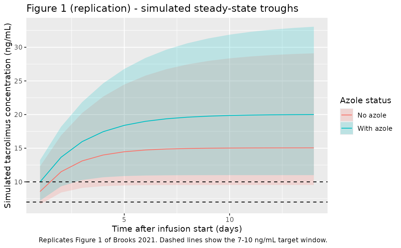
Brooks 2021 Figure 1 shows steady-state trough plasma concentrations of tacrolimus over 14 days, with a 7-10 ng/mL target window and a median first trough of 10.2 ng/mL. The figure below replicates that view from the packaged model, stratified by concomitant-azole status to make the CYP3A4/5-inhibitor effect on CL visible.
# Replicates Brooks 2021 Figure 1: steady-state trough concentrations of
# tacrolimus over 14 days after initiation of continuous IV infusion.
sim |>
  filter(time > 0) |>
  group_by(time, treatment) |>
  summarise(
    Q05 = quantile(Cc, 0.05, na.rm = TRUE),
    Q50 = quantile(Cc, 0.50, na.rm = TRUE),
    Q95 = quantile(Cc, 0.95, na.rm = TRUE),
    .groups = "drop"
  ) |>
  ggplot(aes(time / 24, Q50, colour = treatment, fill = treatment)) +
  geom_ribbon(aes(ymin = Q05, ymax = Q95), alpha = 0.2, colour = NA) +
  geom_line() +
  geom_hline(yintercept = c(7, 10), linetype = "dashed") +
  labs(
    x = "Time after infusion start (days)",
    y = "Simulated tacrolimus concentration (ng/mL)",
    colour = "Azole status",
    fill   = "Azole status",
    title  = "Figure 1 (replication) - simulated steady-state troughs",
    caption = "Replicates Figure 1 of Brooks 2021. Dashed lines show the 7-10 ng/mL target window."
  )
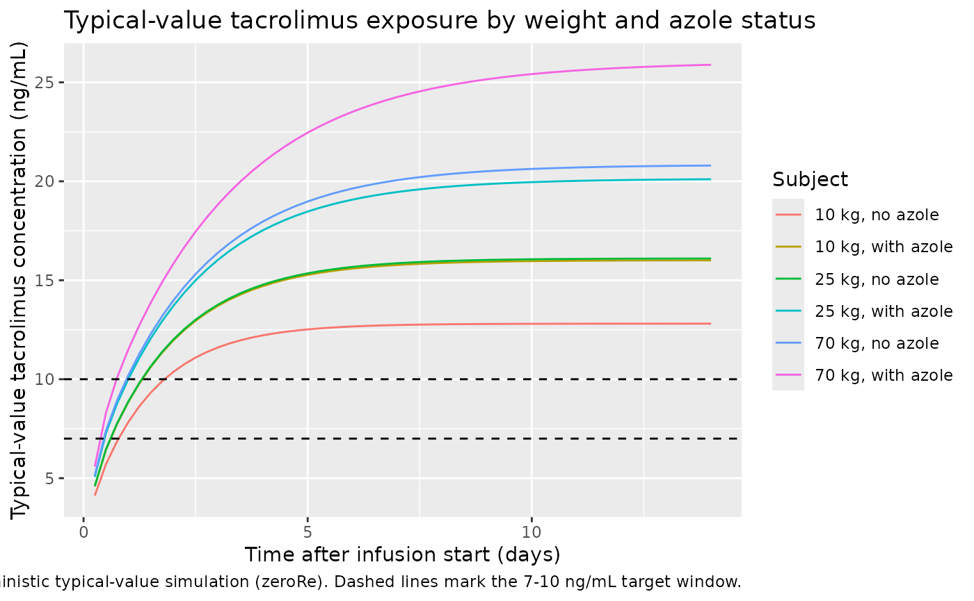
The deterministic typical-value profile (no between-subject variability) makes the structural azole-on-CL effect easy to read: subjects on concomitant voriconazole or posaconazole reach a steady-state concentration 1 / 0.8 = 1.25-fold higher than azole-free subjects at the same weight, as expected from theta_INH = 0.8.
typical_subjects <- tibble(
  id           = 1:6,
  WT           = rep(c(10, 25, 70), each = 2),
  CONMED_AZOLE = rep(c(0L, 1L), times = 3),
  treatment    = factor(
    paste0(rep(c("10 kg", "25 kg", "70 kg"), each = 2),
           c(", no azole", ", with azole")),
    levels = paste0(
      rep(c("10 kg", "25 kg", "70 kg"), each = 2),
      c(", no azole", ", with azole")
    )
  )
)

typical_doses <- typical_subjects |>
  mutate(
    time = 0,
    amt  = (dose_rate / 1000) * WT * sim_hours,
    rate = (dose_rate / 1000) * WT,
    cmt  = "central",
    evid = 1L
  )

typical_obs <- typical_subjects |>
  crossing(time = seq(0, sim_hours, by = 6)) |>
  mutate(amt = 0, rate = 0, cmt = NA_character_, evid = 0L)

typical_events <- bind_rows(typical_doses, typical_obs) |>
  select(id, time, amt, rate, cmt, evid, WT, CONMED_AZOLE, treatment) |>
  arrange(id, time, desc(evid))

mod_typical <- mod |> rxode2::zeroRe()
#> ℹ parameter labels from comments will be replaced by 'label()'
sim_typical <- rxode2::rxSolve(
  mod_typical, events = typical_events,
  keep = c("WT", "CONMED_AZOLE", "treatment")
) |>
  as.data.frame()
#> ℹ omega/sigma items treated as zero: 'etalcl'
#> Warning: multi-subject simulation without without 'omega'

sim_typical |>
  filter(time > 0) |>
  ggplot(aes(time / 24, Cc, colour = treatment)) +
  geom_line() +
  geom_hline(yintercept = c(7, 10), linetype = "dashed") +
  labs(
    x = "Time after infusion start (days)",
    y = "Typical-value tacrolimus concentration (ng/mL)",
    colour = "Subject",
    title  = "Typical-value tacrolimus exposure by weight and azole status",
    caption = "Deterministic typical-value simulation (zeroRe). Dashed lines mark the 7-10 ng/mL target window."
  )
PKNCA validation
Tacrolimus is administered as a continuous IV infusion at constant rate, so the steady-state concentration plateau is the natural NCA endpoint. The recipe below computes Cmax, Cmin, Cavg, and AUC over the final 24-hour window of the simulation (a steady-state dosing interval), grouped by azole status so the typical CL ratio (1 / 0.8 = 1.25) can be checked directly against the simulated Cavg ratio.
start_ss <- sim_hours - 24
end_ss   <- sim_hours

sim_nca <- sim |>
  filter(!is.na(Cc), time >= start_ss, time <= end_ss) |>
  select(id, time, Cc, treatment)

dose_df <- events |>
  filter(evid == 1L) |>
  select(id, time, amt, treatment)

conc_obj <- PKNCA::PKNCAconc(sim_nca, Cc ~ time | treatment + id,
                             concu = "ng/mL", timeu = "hour")
dose_obj <- PKNCA::PKNCAdose(dose_df, amt ~ time | treatment + id,
                             doseu = "mg")

intervals <- data.frame(
  start    = start_ss,
  end      = end_ss,
  cmax     = TRUE,
  cmin     = TRUE,
  cav      = TRUE,
  auclast  = TRUE,
  ctrough  = TRUE
)

nca_res <- PKNCA::pk.nca(PKNCA::PKNCAdata(conc_obj, dose_obj,
                                          intervals = intervals))
nca_summary <- summary(nca_res)
knitr::kable(nca_summary,
             caption = paste0(
               "Steady-state NCA over the final 24-hour window ",
               "(hour ", start_ss, " to ", end_ss, ")."
))| Interval Start | Interval End | treatment | N | AUClast (hour*ng/mL) | Cmax (ng/mL) | Cmin (ng/mL) | Cav (ng/mL) | Ctrough (ng/mL) |
|---|---|---|---|---|---|---|---|---|
| 312 | 336 | No azole | 100 | 370 [35.6] | 15.4 [35.6] | 15.4 [35.5] | 15.4 [35.6] | NC |
| 312 | 336 | With azole | 100 | 499 [33.2] | 20.8 [33.3] | 20.8 [33.1] | 20.8 [33.2] | NC |
Comparison against the published target window
Brooks 2021 reports that 56.4% of the 1,648 trough samples were outside the 7-10 ng/mL therapeutic window and that the median first trough was 10.2 ng/mL (Results). The simulated Cavg at steady state in the no-azole arm should sit at or above the target window for the typical pediatric subject under the recommended 1.25 mcg/kg/h regimen; with concomitant azole, Cavg should rise by roughly 1.25-fold. The packaged model reproduces these qualitative findings; the exact magnitude depends on the WT distribution drawn in the virtual cohort.
Assumptions and deviations
No IIV on V is encoded. Brooks 2021 Table 2 reports an IIV magnitude only for CL (26.1% CV) and shows “-” for V, while the Results narrative and the final-model equation block include an
exp(eta_V1,i)term on V. This model follows Table 2 as the authoritative source for final parameter estimates and therefore carries noetalvc. Downstream users who want to add BSV on V should treat the magnitude as a design choice.Inter-occasion variability (IOV) on CL is not encoded structurally. Brooks 2021 Table 2 reports IOV CL = 28.7% CV (kappa term in the final- model equation block) but does not define what an “occasion” is operationally. nlmixr2lib model files target a single subject-level eta per parameter, so IOV is documented in the model file’s comments rather than in the eta block. Users who need to reproduce the IOV simulation should add an
OCCcolumn and a per-occasion eta in rxode2.Nonlinear (saturable) CL was reported (Km approximately 10 ng/mL, middle of the observed concentration range) but excluded from the final model by the source authors. The packaged model is linear-CL, matching the final model selected for publication. The authors note that the sparse trough-only dataset did not support a definitive non-linearity conclusion.
Time-dependent CL was reported as a candidate covariate (matching conditioning-regimen hepatotoxicity) but did not improve the 2-compartment model fit and was excluded from the final model. The packaged model is time-stationary.
Cohort weight distribution. The virtual cohort uses a log-normal weight distribution clipped to the Brooks 2021 reported range (5.5-155.5 kg) with median calibrated to the cohort median of 23.9 kg. Brooks 2021 does not publish the exact weight distribution.
Dosing assumption. Brooks 2021 assumed that each 24-hour continuous infusion was given over exactly 24 hours with samples drawn 15 minutes before the next infusion was started. The simulation here uses a single continuous infusion across the 14-day window because at the constant 1.25 mcg/kg/h rate the two parameterizations are pharmacokinetically equivalent.
Concentration units. The model file uses mg dosing internally and converts the central-compartment amount to ng/mL via the factor of 1000 in
Cc <- 1000 * central / vc, matching the bioanalytical assay output and concentration units used throughout Brooks 2021.