Glibenclamide whole-body PET microdose (Comin 2025)
Source:vignettes/articles/Comin_2025_glibenclamide.Rmd
Comin_2025_glibenclamide.RmdModel and source
- Citation: Comin L, Marie S, Ursino M, Zohar S, Tournier N, Comets E. Modeling Whole-Body Dynamic PET Microdosing Data to Predict the Whole-Body Pharmacokinetics of Glyburide in Humans. Clin Pharmacokinet. 2025;64(11):1709-1722. doi:10.1007/s40262-025-01562-9 (PMC12618397).
- Description: Seven-compartment semi-physiological population PK model for intravenous microdose [11C]glibenclamide (glyburide) in healthy adult volunteers, fitted to whole-body dynamic PET concentrations in arterial blood, liver, kidneys, spleen and pancreas over the first 40 min after injection. Blood (central) exchanges first-order with a liver compartment and a kidney compartment (each with a catenary deep sub-compartment, the two sub-compartments sharing one organ volume) and with one-compartment spleen and pancreas; first-order elimination from blood; the dose enters blood as a zero-order input of estimated duration. A single intravenous rifampicin dose (OATP inhibition) multiplies the liver-to-blood rate constant by exp(0.96) = 2.6. Inter-occasion variability on that rate constant is fixed (SD 0.01).
- Article: https://doi.org/10.1007/s40262-025-01562-9 (open access, PMC12618397)
Comin et al. fitted a population PK model, in Monolix, to whole-body dynamic PET data acquired over 40 min after an intravenous microdose of [11C]glibenclamide (glyburide; the INN is used here). Concentrations were derived from the image radioactivity in arterial blood, liver, kidneys, spleen and pancreas. Each volunteer was scanned once with the tracer alone and, in 10 of 16, a second time immediately after a 30-min intravenous infusion of rifampicin 9 mg/kg, which inhibits hepatic OATP uptake transporters.
Population
Sixteen healthy volunteers (11 men, 5 women) were enrolled in three groups (Comin 2025 Table 1): men older than 50 years (n = 4, median age 59 years, range 50-64; median weight 81 kg), women older than 50 years (n = 5, 60 years, 59-65; 66 kg) and men younger than 30 years (n = 7, 25 years, 20-30; 73 kg). One woman homozygous for the SLCO1B1 c.521T>C variant (CC genotype) was excluded from model building, so the final model was fitted to 15 subjects; Supplementary Table S1 refits the same model with her included. One man had undergone a splenectomy and contributed no spleen data. The injected microdose was 12.5 +/- 6.2 ug.
The same information is available programmatically via
readModelDb("Comin_2025_glibenclamide")()$population.
Model structure
Results equation 5 and Figure 3 of the paper. All states are amounts
(ug); central is blood.
-
central(blood, volumevc) exchanges first-order withliver,kidney,spleenandpancreasand is the only site of elimination (kel). -
liverexchanges with a catenaryliver_deepsub-compartment;kidneylikewise withkidney_deep. Each organ is observed as the sum of its two sub-compartments divided by one organ volume (v_liver,v_kidney). - The dose enters blood as a zero-order input of estimated duration
Tk0 (
d1= 0.015 h, about 54 s), so dose records userate = -2. - Rifampicin (
CONMED_RIFAMPICIN_SD = 1) multiplies the liver-to-blood rate constantk_liver_centralbyexp(0.96)= 2.61. - Inter-occasion variability (
OCC= 1 or 2) is onk_liver_centralonly, with its SD fixed at 0.01.
Source trace
All values are from Comin 2025 Table 2 (final population estimates). IIV is reported as the SD (omega) of the log-scale random effect; the model carries omega squared.
| Parameter | Paper symbol | Value | Source location |
|---|---|---|---|
lvc |
VB | 3.6 L | Table 2 |
lkel |
ke | 0.79 1/h | Table 2 |
ld1 |
Tk0 | 0.015 h | Table 2 |
lv_liver |
VL | 1.1 L | Table 2 |
lk_liver_central |
kL1B | 21 1/h | Table 2 |
e_conmed_rifampicin_sd_k_liver_central |
beta L1B,Rif | 0.96 | Table 2; legend equation for kL1B,i,o |
lk_central_liver |
kBL1 | 9.0 1/h | Table 2 |
lk_liver_liver_deep |
kL1L2 | 8.2 1/h | Table 2 |
lk_liver_deep_liver |
kL2L1 | 4.5 1/h | Table 2 |
lv_kidney |
VK | 1.6 L | Table 2 |
lk_kidney_central |
kK1B | 179 1/h | Table 2 |
lk_central_kidney |
kBK1 | 62 1/h | Table 2 |
lk_kidney_kidney_deep |
kK1K2 | 19 1/h | Table 2 |
lk_kidney_deep_kidney |
kK2K1 | 8.2 1/h | Table 2 |
lv_spleen |
VS | 0.34 L | Table 2 |
lk_central_spleen |
kBS | 5.9 1/h | Table 2 |
lk_spleen_central |
kSB | 131 1/h | Table 2 |
lv_pancreas |
VP | 0.23 L | Table 2 |
lk_central_pancreas |
kBP | 5.9 1/h | Table 2 |
lk_pancreas_central |
kPB | 138 1/h | Table 2 |
etalvc, etalkel, etald1
|
omega VB, ke, Tk0 | 0.18, 0.35, 0.46 (SD) | Table 2 |
etalv_liver, etalk_liver_central,
etalk_central_liver,
etalk_liver_deep_liver
|
omega VL, L1B, BL1, L2L1 | 0.54, 0.22, 0.40, 0.22 (SD) | Table 2 |
etalv_kidney, etalk_central_kidney,
etalk_kidney_kidney_deep,
etalk_kidney_deep_kidney
|
omega VK, BK1, K1K2, K2K1 | 0.091, 0.26, 0.15, 0.12 (SD) | Table 2 |
etalk_central_spleen |
omega BS | 0.20 (SD) | Table 2 |
etalk_central_pancreas,
etalk_pancreas_central
|
omega BP, PB | 0.38, 0.30 (SD) | Table 2 |
etaiov_lk_liver_central_1, _2
|
gamma kL1B | 0.01 (SD), fixed | Results; Table 2 legend |
addSd, propSd
|
aB, bB | 0.062 ug/L, 0.26 | Table 2 (combined error) |
addSd_Cliver |
aL | 0.12 ug/L | Table 2 (constant error) |
addSd_Ckidney |
aK | 0.23 ug/L | Table 2 (constant error) |
addSd_Cspleen, propSd_Cspleen
|
aS, bS | 0.038 ug/L, 0.24 | Table 2 (combined error) |
addSd_Cpancreas, propSd_Cpancreas
|
aP, bP | 0.026 ug/L, 0.19 | Table 2 (combined error) |
| ODE system and organ concentrations | Results equation 5; Figure 3 | ||
| Combined error form g = a + b f | Methods, Statistical Model |
Derived quantities stated in the paper
The Results and Discussion quote several quantities that follow directly from the Table 2 estimates. They are recomputed here from the packaged model; the two sides are the same arithmetic, so the tolerances only absorb the paper’s rounding.
mod <- readModelDb("Comin_2025_glibenclamide")
ui <- rxode2::rxode(mod)
#> ℹ parameter labels from comments will be replaced by 'label()'
#> Warning: some etas defaulted to non-mu referenced, possible parsing error: etaiov_lk_liver_central_1, etaiov_lk_liver_central_2
#> as a work-around try putting the mu-referenced expression on a simple line
th <- ui$theta

cl <- exp(th[["lvc"]]) * exp(th[["lkel"]])
k_lb <- exp(th[["lk_liver_central"]])
k_lb_rif <- k_lb * exp(th[["e_conmed_rifampicin_sd_k_liver_central"]])
k_bl <- exp(th[["lk_central_liver"]])
k_kb <- exp(th[["lk_kidney_central"]])
k_bk <- exp(th[["lk_central_kidney"]])
v_tissue <- exp(th[["lv_liver"]]) + exp(th[["lv_kidney"]]) +
  exp(th[["lv_spleen"]]) + exp(th[["lv_pancreas"]])

derived <- tibble::tribble(
  ~quantity, ~model, ~paper, ~where,
  "CL = VB x ke (L/h)", cl, 2.84, "Results",
  "kL1B with rifampicin (1/h)", k_lb_rif, 55, "Results; Discussion",
  "kL1B / kBL1, no rifampicin", k_lb / k_bl, 2.3, "Results",
  "kK1B / kBK1", k_kb / k_bk, 2.9, "Results",
  "kBL1 / kL1B, no rifampicin", k_bl / k_lb, 0.43, "Discussion",
  "kBL1 / kL1B, with rifampicin", k_bl / k_lb_rif, 0.16, "Discussion",
  "Sum of organ volumes except blood (L)", v_tissue, 3.3, "Discussion"
) |>
  mutate(pct_diff = 100 * (model - paper) / paper)

derived |>
  dplyr::rename(
    "Quantity" = quantity, "Model" = model, "Paper" = paper,
    "Paper location" = where, "% difference" = pct_diff
  ) |>
knitr::kable(digits = c(0, 3, 2, 0, 1))| Quantity | Model | Paper | Paper location | % difference |
|---|---|---|---|---|
| CL = VB x ke (L/h) | 2.844 | 2.84 | Results | 0.1 |
| kL1B with rifampicin (1/h) | 54.846 | 55.00 | Results; Discussion | -0.3 |
| kL1B / kBL1, no rifampicin | 2.333 | 2.30 | Results | 1.4 |
| kK1B / kBK1 | 2.887 | 2.90 | Results | -0.4 |
| kBL1 / kL1B, no rifampicin | 0.429 | 0.43 | Discussion | -0.3 |
| kBL1 / kL1B, with rifampicin | 0.164 | 0.16 | Discussion | 2.6 |
| Sum of organ volumes except blood (L) | 3.270 | 3.30 | Discussion | -0.9 |
Typical-value profiles (Figure 4)
Figure 4 of the paper shows individual fits for three subjects in each tissue on both occasions. The typical-value predictions below show the same pattern: the blood peak at the end of the short input followed by a rapid fall, liver concentrations still rising at 40 min, kidney peaking at about 10 min, and fast blood equilibrium in spleen and pancreas. Rifampicin roughly halves the liver concentration and raises blood, kidney, spleen and pancreas concentrations a little.
dose_ug <- 12.5
t_obs <- sort(unique(c(seq(0, 3 / 60, by = 10 / 3600), seq(3 / 60, 40 / 60, by = 2.5 / 60))))

make_events <- function(ids, occ, rif) {
  dose <- tibble(
    id = ids, time = 0, amt = dose_ug, rate = -2, evid = 1L,
    cmt = "central", dvid = NA_integer_
  )
  obs <- tidyr::crossing(id = ids, time = t_obs) |>
    mutate(amt = 0, rate = 0, evid = 0L, cmt = "central", dvid = 1L)
  bind_rows(dose, obs) |>
    mutate(OCC = occ, CONMED_RIFAMPICIN_SD = rif) |>
    arrange(id, time, desc(evid))
}

ev_typ <- bind_rows(
  make_events(1L, occ = 1L, rif = 0L) |> mutate(occasion = "Baseline"),
  make_events(2L, occ = 2L, rif = 1L) |> mutate(occasion = "Rifampicin")
)

tissues <- c(Cc = "Blood", Cliver = "Liver", Ckidney = "Kidneys", Cpancreas = "Pancreas", Cspleen = "Spleen")

sim_typ <- rxode2::rxSolve(
  rxode2::zeroRe(mod),
  events = ev_typ, keep = "occasion"
) |>
  as.data.frame()
#> ℹ parameter labels from comments will be replaced by 'label()'
#> Warning: some etas defaulted to non-mu referenced, possible parsing error: etaiov_lk_liver_central_1, etaiov_lk_liver_central_2
#> as a work-around try putting the mu-referenced expression on a simple line
#> Warning: some etas defaulted to non-mu referenced, possible parsing error: etaiov_lk_liver_central_1, etaiov_lk_liver_central_2
#> as a work-around try putting the mu-referenced expression on a simple line
#> ℹ omega/sigma items treated as zero: 'etalvc', 'etalkel', 'etald1', 'etalv_liver', 'etalk_liver_central', 'etalk_central_liver', 'etalk_liver_deep_liver', 'etalv_kidney', 'etalk_central_kidney', 'etalk_kidney_kidney_deep', 'etalk_kidney_deep_kidney', 'etalk_central_spleen', 'etalk_central_pancreas', 'etalk_pancreas_central', 'etaiov_lk_liver_central_1', 'etaiov_lk_liver_central_2'
#> Warning: multi-subject simulation without without 'omega'

sim_typ_long <- sim_typ |>
  select(id, time, occasion, all_of(names(tissues))) |>
  pivot_longer(all_of(names(tissues)), names_to = "output", values_to = "conc") |>
  mutate(tissue = factor(tissues[output], levels = tissues))

ggplot(sim_typ_long, aes(time, conc, colour = occasion)) +
  geom_line() +
  facet_wrap(~tissue, nrow = 1, scales = "free_y") +
  labs(
    x = "Time (h)", y = "Concentration (ug/L)", colour = NULL,
    title = "Typical-value profiles after 12.5 ug [11C]glibenclamide",
    caption = "Compare with the individual fits in Figure 4 of Comin 2025."
  ) +
  theme(legend.position = "bottom")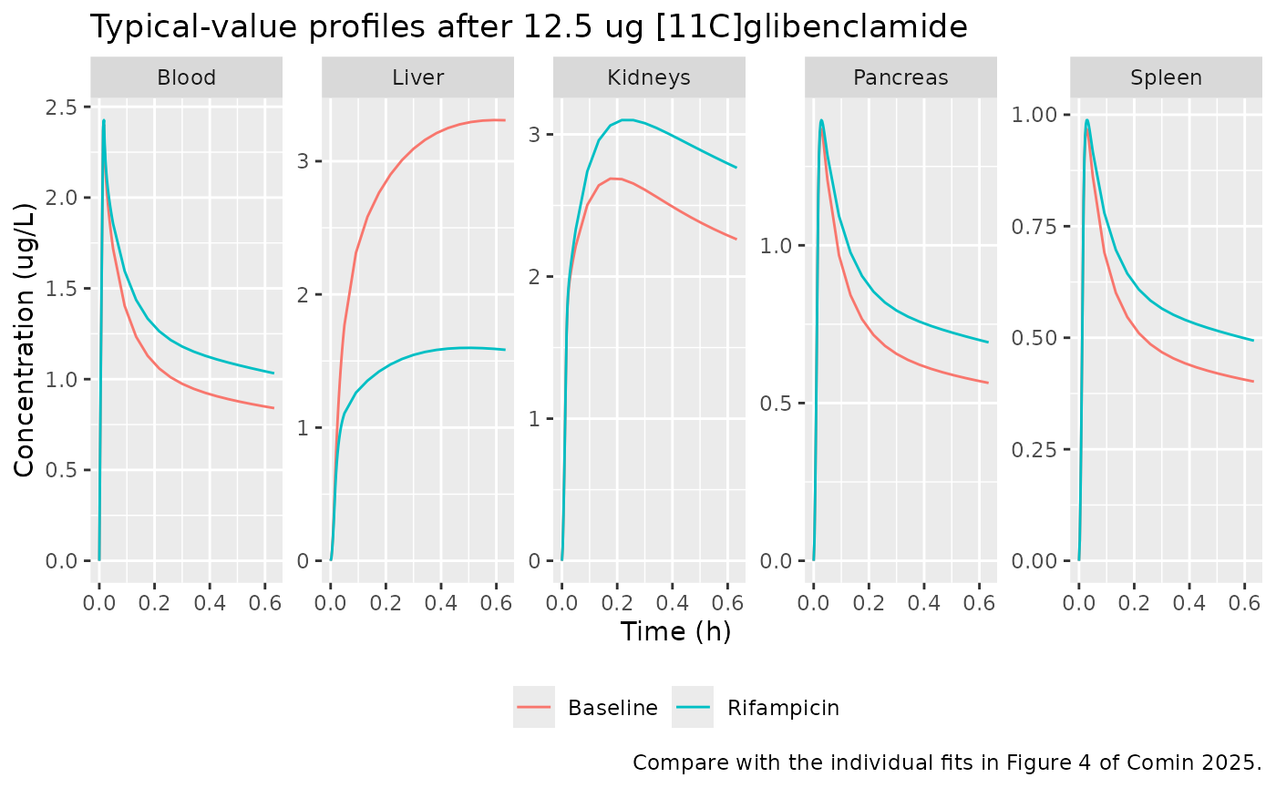
Mass balance
Without a sink other than kel, the amount still in the
body plus the cumulative elimination must equal the dose. The cumulative
elimination is the trapezoidal integral of kel * central on
a fine grid, so the check is limited only by quadrature error.
ev_mb <- make_events(1L, occ = 1L, rif = 0L) |>
  filter(evid == 1L) |>
  bind_rows(tibble(
    id = 1L, time = seq(0, 3, by = 1 / 3600), amt = 0, rate = 0, evid = 0L,
    cmt = "central", dvid = 1L, OCC = 1L, CONMED_RIFAMPICIN_SD = 0L
  ))

mb <- rxode2::rxSolve(rxode2::zeroRe(mod), events = ev_mb) |>
  as.data.frame() |>
  mutate(
    in_body = central + liver + liver_deep + kidney + kidney_deep + spleen + pancreas,
    elim_rate = exp(th[["lkel"]]) * central,
    eliminated = c(0, cumsum(diff(time) * (head(elim_rate, -1) + tail(elim_rate, -1)) / 2)),
    total = in_body + eliminated
  )
#> ℹ parameter labels from comments will be replaced by 'label()'
#> Warning: some etas defaulted to non-mu referenced, possible parsing error: etaiov_lk_liver_central_1, etaiov_lk_liver_central_2
#> as a work-around try putting the mu-referenced expression on a simple line
#> Warning: some etas defaulted to non-mu referenced, possible parsing error: etaiov_lk_liver_central_1, etaiov_lk_liver_central_2
#> as a work-around try putting the mu-referenced expression on a simple line
#> ℹ omega/sigma items treated as zero: 'etalvc', 'etalkel', 'etald1', 'etalv_liver', 'etalk_liver_central', 'etalk_central_liver', 'etalk_liver_deep_liver', 'etalv_kidney', 'etalk_central_kidney', 'etalk_kidney_kidney_deep', 'etalk_kidney_deep_kidney', 'etalk_central_spleen', 'etalk_central_pancreas', 'etalk_pancreas_central', 'etaiov_lk_liver_central_1', 'etaiov_lk_liver_central_2'

mb_err <- max(abs(mb$total[mb$time >= 0.1] - dose_ug)) / dose_ug
mb_err
#> [1] 6.932944e-09
stopifnot(mb_err < 0.005)
Stochastic simulation (Supplementary Figure S2)
Supplementary Figure S2 is a prediction-corrected VPC with the 10th, 50th and 90th percentiles. The simulation below uses 200 virtual subjects per occasion, each receiving the mean microdose of 12.5 ug, with between-subject and residual variability.
rxode2::rxSetSeed(20251)
n_per_occ <- 200L
ev_vpc <- bind_rows(
  make_events(seq_len(n_per_occ), occ = 1L, rif = 0L) |>
    mutate(occasion = "Baseline"),
  make_events(n_per_occ + seq_len(n_per_occ), occ = 2L, rif = 1L) |>
    mutate(occasion = "Rifampicin")
)
stopifnot(!anyDuplicated(unique(ev_vpc[, c("id", "time", "evid")])))

sim <- rxode2::rxSolve(mod, events = ev_vpc, keep = "occasion") |>
  as.data.frame()
#> ℹ parameter labels from comments will be replaced by 'label()'
#> Warning: some etas defaulted to non-mu referenced, possible parsing error: etaiov_lk_liver_central_1, etaiov_lk_liver_central_2
#> as a work-around try putting the mu-referenced expression on a simple line

vpc <- sim |>
  select(id, time, occasion, all_of(names(tissues))) |>
  pivot_longer(all_of(names(tissues)), names_to = "output", values_to = "conc") |>
  mutate(tissue = factor(tissues[output], levels = tissues)) |>
  group_by(tissue, occasion, time) |>
  summarise(
    p10 = quantile(conc, 0.10), p50 = quantile(conc, 0.50), p90 = quantile(conc, 0.90),
    .groups = "drop"
  )

ggplot(vpc, aes(time, p50, colour = occasion, fill = occasion)) +
  geom_ribbon(aes(ymin = p10, ymax = p90), alpha = 0.2, colour = NA) +
  geom_line() +
  facet_wrap(~tissue, nrow = 1, scales = "free_y") +
  labs(
    x = "Time (h)", y = "Concentration (ug/L)", colour = NULL, fill = NULL,
    title = "Simulated median and 10th-90th percentiles (IPRED)",
    caption = "Compare with Supplementary Figure S2 of Comin 2025."
  ) +
  theme(legend.position = "bottom")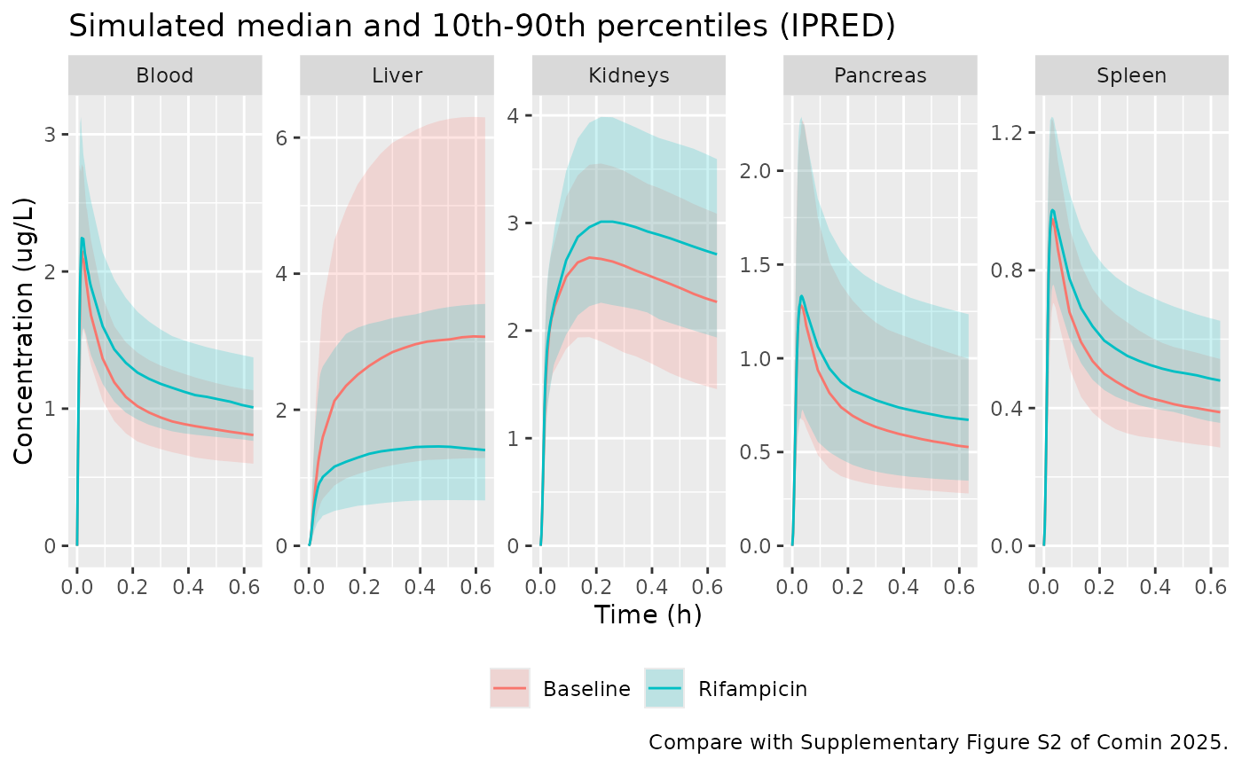
PKNCA: exposure over the 40-min acquisition
The paper does not tabulate NCA values. The companion
non-compartmental analysis of the same data (Marie et al., cited as
reference 6) is quoted in the Discussion as a blood AUC increase of +24
+/- 24% with rifampicin. PKNCA is run below on the individual
predictions (the Cc and Cliver columns that
rxSolve returns, which carry between-subject but not
residual variability) over the 0-40 min acquisition window, by
occasion.
run_nca <- function(dat, output) {
  conc <- dat |>
    filter(!is.na(.data[[output]])) |>
    transmute(id, occasion, time, conc = .data[[output]])
  conc <- bind_rows(
    conc,
    conc |> distinct(id, occasion) |> mutate(time = 0, conc = 0)
  ) |>
    distinct(id, occasion, time, .keep_all = TRUE) |>
    arrange(id, occasion, time)
  doses <- ev_vpc |>
    filter(evid == 1L) |>
    select(id, occasion, time, amt)
  intervals <- data.frame(start = 0, end = 40 / 60, cmax = TRUE, tmax = TRUE, auclast = TRUE)
  PKNCA::pk.nca(PKNCA::PKNCAdata(
    PKNCA::PKNCAconc(conc, conc ~ time | occasion + id),
    PKNCA::PKNCAdose(doses, amt ~ time | occasion + id),
    intervals = intervals
  ))
}

nca_blood <- run_nca(sim, "Cc")
nca_liver <- run_nca(sim, "Cliver")

nca_summary <- bind_rows(
  as.data.frame(nca_blood$result) |> mutate(tissue = "Blood"),
  as.data.frame(nca_liver$result) |> mutate(tissue = "Liver")
) |>
  group_by(tissue, occasion, PPTESTCD) |>
  summarise(median = median(PPORRES), .groups = "drop") |>
  pivot_wider(names_from = PPTESTCD, values_from = median)

nca_summary |>
  select(tissue, occasion, cmax, tmax, auclast) |>
  dplyr::rename(
    "Tissue" = tissue, "Occasion" = occasion, "Cmax (ug/L)" = cmax,
    "Tmax (h)" = tmax, "AUC0-40min (ug*h/L)" = auclast
  ) |>
knitr::kable(digits = 3, caption = "Median simulated NCA over the 40-min acquisition (200 subjects per occasion).")| Tissue | Occasion | Cmax (ug/L) | Tmax (h) | AUC0-40min (ug*h/L) |
|---|---|---|---|---|
| Blood | Baseline | 2.446 | 0.017 | 0.659 |
| Blood | Rifampicin | 2.537 | 0.014 | 0.806 |
| Liver | Baseline | 3.093 | 0.592 | 1.666 |
| Liver | Rifampicin | 1.463 | 0.508 | 0.829 |
auc_ratio <- nca_summary |>
  select(tissue, occasion, auclast) |>
  pivot_wider(names_from = occasion, values_from = auclast) |>
  mutate(pct_change = 100 * (Rifampicin / Baseline - 1))
knitr::kable(auc_ratio, digits = 2, caption = "Rifampicin effect on median AUC0-40min.")| tissue | Baseline | Rifampicin | pct_change |
|---|---|---|---|
| Blood | 0.66 | 0.81 | 22.33 |
| Liver | 1.67 | 0.83 | -50.27 |
The model-predicted blood AUC increase with rifampicin is within the +24 +/- 24% range of the companion NCA, and the liver AUC falls by roughly half, consistent with the paper’s statement that the final model shows “a significant reduction in hepatic radioactivity following OATP inhibition”. The checks below are deliberately loose: the two sides are a model prediction and an independent NCA of observed data, and the blood comparison is between medians of unpaired virtual cohorts.
blood_change <- auc_ratio$pct_change[auc_ratio$tissue == "Blood"]
liver_change <- auc_ratio$pct_change[auc_ratio$tissue == "Liver"]
stopifnot(
  blood_change > 0, blood_change < 48,
  liver_change < -25, liver_change > -75
)
Assumptions and deviations
- Final model only. The paper also reports the final model refitted with the SLCO1B1 CC subject (Supplementary Table S1), an alternative with spleen and pancreas as fixed ratios of blood (Table S2), and a blood + liver-only model (Table S3). These are sensitivity analyses and are not packaged.
- IOV value read as an SD. The paper states that the IOV on kL1B “was fixed at 0.01”. Table 2 reports every other random effect as an SD (omega), as Monolix does, so 0.01 is taken as the SD and the model carries a variance of 1e-4 on each of the two occasion-level random effects.
- Concentration units. The Methods text converts radioactivity to “ug/mL”, but Table 2 gives the additive errors in ug/L, and the dose (about 12.5 ug) divided by the blood volume (3.6 L) gives concentrations of a few ug/L. The model uses ug for amounts, L for volumes and ug/L for concentrations.
- Compartment count. The abstract says the final model has seven compartments and the Results says six; the published equation system (Results equation 5) has seven states (blood, two liver, two kidney, spleen, pancreas), which is what is implemented.
- Covariance. Correlations between random effects were tested but none is reported in Table 2, so all random effects are independent.
- Parent-drug signal. As in the paper, the PET radioactivity is attributed entirely to parent glibenclamide; the authors note radiometabolites were below 10% of blood radioactivity by the end of acquisition.
- Poorly identified spleen and pancreas parameters. VS, kBS, VP and kBP have relative standard errors of order 1e5% in Table 2 and varied three- to eight-fold between estimation runs (Supplementary Figure S3). They are packaged as published; the concentration ratios they imply are better determined than the individual values.
- Microdose. The model describes the first 40 min after a microdose and the authors caution against extrapolating the elimination rate; it is not a model of therapeutic glibenclamide dosing.
- No correction notice for the article was found as of 2026-11-10.