Monoclonal antibody whole-body PBPK (Jones 2019)
Source:vignettes/articles/Jones_2019_mab_pbpk.Rmd
Jones_2019_mab_pbpk.RmdModel and source
- Citation: Jones HM, Zhang Z, Jasper P, Luo H, Avery LB, King LE, Neubert H, Barton HA, Betts AM, Webster R. A Physiologically-Based Pharmacokinetic Model for the Prediction of Monoclonal Antibody Pharmacokinetics From In Vitro Data. CPT Pharmacometrics Syst Pharmacol. 2019;8(10):738-747. doi:10.1002/psp4.12461
- Description: PBPK / QSP (whole-body, 15 organs, 620 ODE states). Platform model predicting human linear pharmacokinetics of an IgG1 monoclonal antibody a priori from two in vitro inputs: an AC-SINS polyspecificity score and the FcRn binding affinity at pH 6.0. Each organ carries vascular, vascular-side membrane, three pH-resolved endosomal transit compartments (early pH 7.4, sorting pH 6.0, recycling pH 7.4), interstitial-side membrane and interstitial space. Dosed antibody and endogenous IgG compete for a shared FcRn pool with explicit 1:1 and 2:1 stoichiometry, and non-specific charge-mediated binding to cell-membrane sites provides an FcRn-independent clearance route driven by the AC-SINS score. Extends the Shah and Betts 2012 platform topology.
- Article: https://doi.org/10.1002/psp4.12461 (open access, PMC6813168)
- Supplement: Tables S1-S3, the “PBPK Model Equations” listing, and the Berkeley Madonna model code (human parameterisation), all distributed with the article.
Jones et al. (2019) built a whole-body PBPK model that predicts the linear pharmacokinetics of an IgG1 monoclonal antibody (mAb) a priori from two in vitro measurements: an AC-SINS self-association score, which drives an FcRn-independent non-specific clearance route, and the FcRn binding affinity at pH 6.0. The organ topology and physiology are those of Shah and Betts (2012). The new part is a mechanistic endothelial cell in every organ. It has a vascular-side membrane, three pH-resolved endosomes in series (early pH 7.4, sorting pH 6.0, recycling pH 7.4) and an interstitial-side membrane. At each location the antibody is free, bound 1:1 to FcRn, or bound 2:1 (one antibody carrying two FcRn). The dosed antibody and endogenous IgG compete for a single FcRn pool.
The main text prints no equations. It defers them to the supplement, and every constant in the model file comes from the deposited Madonna listing, which gives Table 1 and Table 2 at full precision.
mod <- rxode2::rxode(readModelDb("Jones_2019_mab_human_pbpk"))
c(states = length(mod$state))
#> states
#>    620
The model is deterministic. The paper reports no between-subject
variability and no residual-error model, so propSd is fixed
at zero.
Population
Jones et al. calibrated the human model on seven training mAbs (mAbs
1-3 and 5-8) and tested it on five (mAbs 11-14 and 23). Each mAb came
from a single-dose clinical PK study, in-house (Pfizer) or from the
literature, in healthy volunteers or patients, at saturating doses where
PK was linear. Only subcutaneous data were available for mAb 11. The
whole-body catabolic capacity was calibrated jointly against Tg32-mouse
and human profiles, including FcRn-knockout mice and humans with a
beta-2-microglobulin mutation (familial hypercatabolic
hypoproteinaemia). The physiology is a 71 kg adult male (Table S2).
Demographics of the clinical studies are not reported; the model
represents a single reference adult and has no covariates. The same
information is stored in the model’s population
metadata.
Source trace
Every ini() value carries an in-file comment naming its
origin in
inst/modeldb/specificDrugs/Jones_2019_mab_human_pbpk.R. The
table collects them. “Madonna” means the deposited Berkeley Madonna
listing (Supplementary Model Code).
| Parameter / equation | Value | Source location |
|---|---|---|
lendoscale (human / Tg32 endothelial-cell scale) |
603.7 | Madonna human_endo_scale_factor; gives Table 1 human
N_endo = 0.86E12 |
lnendomouse (Tg32 endothelial-cell number) |
1.422E9, fixed | Table 1 (14.2E8); Madonna Total_Endothelial_Cell
|
lkdratio (Kd pH 7.4 / Kd pH 6.0) |
220.11 | Table 1 (220); Madonna KD7_WT / KD6_WT = 154077 /
700 |
lkonratio (first / second FcRn association) |
83.7 | Table 1 |
lkd6 (Kd, pH 6.0) |
700 nM, fixed | Methods, “binding affinity value of 700 nM for pH 6.0” |
lkon6 (k_on, pH 6.0) |
80.6 1/uM/h, fixed | Methods, k_on_1st = 8.06E+7 1/M/h |
lkon7 (k_on, pH 7.4) |
3.22 1/uM/h, fixed | Madonna k_on_7_EXG = 1.61E7 / 5 1/M/h |
lclup (pinocytotic uptake) |
150 nL/h/1E6 cells, fixed | Table 1 |
lpinotime (endosomal transit time) |
0.18 h, fixed | Methods, 10.8 min (Table 1 rounds to 11) |
lfcrntot (total body FcRn) |
1022 nmol, fixed | Table 1 |
lkdegfcrnab (FcRn-bound mAb degradation, pH 7.4) |
ln 2 / 11.1 1/h, fixed | Table 1; Madonna LOGN(2)/11.1
|
probdeg (degradation probability, no FcRn) |
0.95, fixed | Madonna Prob_deg; Table 1 prints 98% (see Errata) |
fr (apical fraction of pinocytosis) |
0.715, fixed | Methods |
frecycle (free-FcRn recycle fraction) |
0.99, fixed | Methods |
sigis (lymph reflection coefficient) |
0.2, fixed | Madonna sigma_IS
|
e6apct (sorting-endosome volume fraction) |
0.33, fixed | Madonna E6a_Vol_Pct
|
tauvm, tauism (membrane residence
times) |
1/60 h, fixed | Madonna tau_VM, tau_ISM
|
cigg0 (endogenous IgG, clamped) |
66.67 uM, fixed | Madonna EDG_mg_ml = 10 mg/mL at MW 150000 |
mwmab (molecular weight) |
150000 g/mol, fixed | Madonna MW_EDG
|
lpsa, lpsb (AC-SINS to Kd scaling) |
1.8051, 0.2624 | Table 2 human (1.81, -0.262); Madonna PS_a,
PS_b
|
lcmem (membrane site density) |
18.5 uM | Table 2 |
lkintps (internalisation of membrane-bound mAb) |
0.0380 1/h | Table 2 human |
lka, fsc (SC absorption,
bioavailability) |
0.26 1/day, 0.60, fixed | Madonna ka, F (see Errata) |
psscore (AC-SINS score of the simulated mAb) |
0, fixed | Madonna PS_Score; assay range 0-25 |
| Organ volumes, plasma flows, reflection coefficients, FcRn fractions | per organ | Table S2; Madonna organ vectors |
| Lymph flow = 0.2% of plasma flow; liver receives splanchnic outflow | n/a | Methods; Madonna LF[LIVER]
|
log10 Kd_PS = exp(PS_a - PS_b * PS_Score) |
n/a | Methods; Supplement “Binding affinity from polyspecificity” |
Endosomal volume V_endo = CL_up * T_endo; FcRn conc. =
amount / V_endo |
n/a | Methods |
| Per-organ vascular, membrane, endosome, interstitial ODEs | n/a | Supplement “PBPK Model Equations”; Madonna
d/dt(C_EXG[...]), d/dt(C_EDG[...]),
d/dt(C_FcRn_*)
|
Observation Cc = c_central * MW / 1000 (ug/mL) |
n/a | Unit conversion; the published figures plot ug/mL |
Madonna integrates concentrations and divides each flux sum by a
volume. The model file integrates amounts, so each d/dt()
is the Madonna numerator written out term by term. The two forms are
exactly equivalent.
Derived constants reproduce the numbers stated in the paper
Several quantities in the paper are outputs of the constants
above, stated separately from them. They are computed inside
model(), so a single solve returns them.
dose_mgkg <- 5 # Madonna Dose_in_mgkg
bw <- 71 # Table S2 reference adult
dose_umol <- dose_mgkg * bw / 150000 * 1000

ev_typ <- et(amt = dose_umol, cmt = "central") |>
  et(sort(unique(c(0, 0.25, 0.5, 1, 2, 4, 8, seq(12, 5000, by = 12)))))
sim_typ <- as.data.frame(rxSolve(mod, ev_typ))

d0 <- sim_typ[1, ]
derived <- tibble::tribble(
  ~quantity, ~model, ~paper, ~source,
  "Endosomal FcRn concentration (uM)", d0$fcrnconc, 44.1, "Methods",
  "Human endothelial-cell number (x1E12)", d0$nendo / 1e12, 0.86, "Table 1",
  "Second FcRn association rate (1/M/h, x1E5)", d0$kon6b * 1e6 / 1e5, 9.63, "Methods",
  "Kd pH 7.4 / Kd pH 6.0", d0$kd7 / d0$kd6, 220, "Table 1"
) |>
  mutate(pct_diff = 100 * (model / paper - 1))
knitr::kable(derived, digits = c(0, 4, 4, 0, 2))| quantity | model | paper | source | pct_diff |
|---|---|---|---|---|
| Endosomal FcRn concentration (uM) | 44.0927 | 44.10 | Methods | -0.02 |
| Human endothelial-cell number (x1E12) | 0.8585 | 0.86 | Table 1 | -0.18 |
| Second FcRn association rate (1/M/h, x1E5) | 9.6296 | 9.63 | Methods | 0.00 |
| Kd pH 7.4 / Kd pH 6.0 | 220.1100 | 220.00 | Table 1 | 0.05 |
All four agree with the paper to its printed precision.
FcRn mass balance
FcRn is neither synthesised nor degraded in this model, so the total receptor (free, plus one per 1:1 complex, plus two per 2:1 complex, over both antibodies and all 75 organ locations) must stay equal to Table 1’s 1022 nmol for the whole solve (Table 1’s figure plus the small membrane seed described in the chunk). The balance tests the model’s topology: a flux sent to the wrong state, or a 2:1 complex counted with the wrong weight, shows up as drift.
cols <- names(sim_typ)
free_fcrn <- grep("^fcrn(memvas|memint|endoearly|endosort|endorecyc)_", cols, value = TRUE)
fr1 <- grep("^(memvas|memint|endoearly|endosort|endorecyc)fr1_", cols, value = TRUE)
fr2 <- grep("^(memvas|memint|endoearly|endosort|endorecyc)fr2_", cols, value = TRUE)
c(free = length(free_fcrn), complex_1to1 = length(fr1), complex_2to1 = length(fr2))
#>         free complex_1to1 complex_2to1
#>           75          150          150

fcrn_total_nmol <- 1000 * (rowSums(sim_typ[, free_fcrn]) +
  rowSums(sim_typ[, fr1]) + 2 * rowSums(sim_typ[, fr2]))
fcrn_summary <- c(
  initial_nmol = fcrn_total_nmol[1],
  max_rel_drift = max(abs(fcrn_total_nmol / fcrn_total_nmol[1] - 1))
)
fcrn_summary
#>  initial_nmol max_rel_drift
#>  1.022019e+03  8.672851e-11
# The 1022 nmol of Table 1 is distributed over the endosomes; the two
# membranes are seeded on top of it at 1e-4 of the endosomal concentration
# (Madonna INIT block), which adds about 0.02 nmol. Drift compares the solve
# with itself, so the only difference is numerical error and a tight bound is
# correct here.
stopifnot(
  abs(fcrn_total_nmol[1] / 1022 - 1) < 1e-4,
  fcrn_summary[["max_rel_drift"]] < 1e-6
)
Replicate Figure 2b: typical human IgG1, with and without FcRn
Figure 2b shows the calibrated human profile of a typical IgG1 and the profile of a human with non-functional FcRn. The curves below were digitised from the vector graphics of the published figure. Figure 2 gives no dose.
fig2 <- tibble::tribble(
  ~panel, ~time, ~Cc_pub,
  "Wild type", 24, 51.3,
  "Wild type", 168, 36.0,
  "Wild type", 336, 27.3,
  "Wild type", 672, 17.0,
  "Wild type", 1000, 11.1,
  "Wild type", 1500, 5.87,
  "Wild type", 2000, 3.12,
  "Wild type", 2500, 1.66,
  "Wild type", 3000, 0.905,
  "Wild type", 3500, 0.483,
  "Wild type", 4000, 0.255,
  "Wild type", 4500, 0.138,
  "FcRn deficient", 24, 53.2,
  "FcRn deficient", 48, 41.9,
  "FcRn deficient", 96, 26.8,
  "FcRn deficient", 168, 14.3,
  "FcRn deficient", 250, 7.31,
  "FcRn deficient", 336, 3.73,
  "FcRn deficient", 400, 2.27,
  "FcRn deficient", 500, 1.1
)
FcRn deficiency is represented by setting the total body FcRn close to zero. The paper does not state how its knockout arm was parameterised; this is the direct reading.
ev_ko <- et(amt = dose_umol, cmt = "central") |>
  et(sort(unique(c(0, 0.25, 0.5, 1, 2, 4, 8, seq(12, 1000, by = 4)))))
sim_ko <- as.data.frame(rxSolve(mod, ev_ko, params = c(lfcrntot = log(1e-6))))

sim_fig2 <- bind_rows(
  sim_typ |> transmute(panel = "Wild type", time, Cc),
  sim_ko |> transmute(panel = "FcRn deficient", time, Cc)
)
cmp2 <- inner_join(fig2, sim_fig2, by = c("panel", "time")) |>
  mutate(ratio = Cc_pub / Cc)
cmp2_summary <- cmp2 |>
  group_by(panel) |>
  summarise(
    median_ratio = median(ratio),
    ratio_cv_pct = 100 * sd(ratio) / mean(ratio),
    .groups = "drop"
  )
knitr::kable(cmp2_summary, digits = 3)| panel | median_ratio | ratio_cv_pct |
|---|---|---|
| FcRn deficient | 0.995 | 3.059 |
| Wild type | 0.812 | 0.809 |
The published wild-type curve equals the model curve multiplied by a constant (coefficient of variation of the ratio under 1% from 24 h to 4500 h). The shape, including the terminal half-life, is therefore identical, and only the unstated dose differs: the constant implies about 4.06 mg/kg against the 5 mg/kg simulated here. The FcRn-deficient curve matches in absolute terms at the deposited 5 mg/kg.
wt <- cmp2_summary[cmp2_summary$panel == "Wild type", ]
ko <- cmp2 |> filter(panel == "FcRn deficient")
stopifnot(
  wt$ratio_cv_pct < 3,
  all(abs(ko$ratio - 1) < 0.1)
)
fig2_plot <- fig2 |>
  left_join(cmp2_summary, by = "panel") |>
  mutate(Cc_plot = if_else(panel == "Wild type", Cc_pub / median_ratio, Cc_pub))
ggplot(sim_fig2[sim_fig2$time > 0 & sim_fig2$Cc > 0.1, ], aes(time, Cc, colour = panel)) +
  geom_line() +
  geom_point(data = fig2_plot, aes(y = Cc_plot), shape = 1, size = 2) +
  scale_y_log10(limits = c(0.1, 1000)) +
  labs(x = "Time (h)", y = "Plasma concentration (ug/mL)", colour = NULL) +
  theme_bw()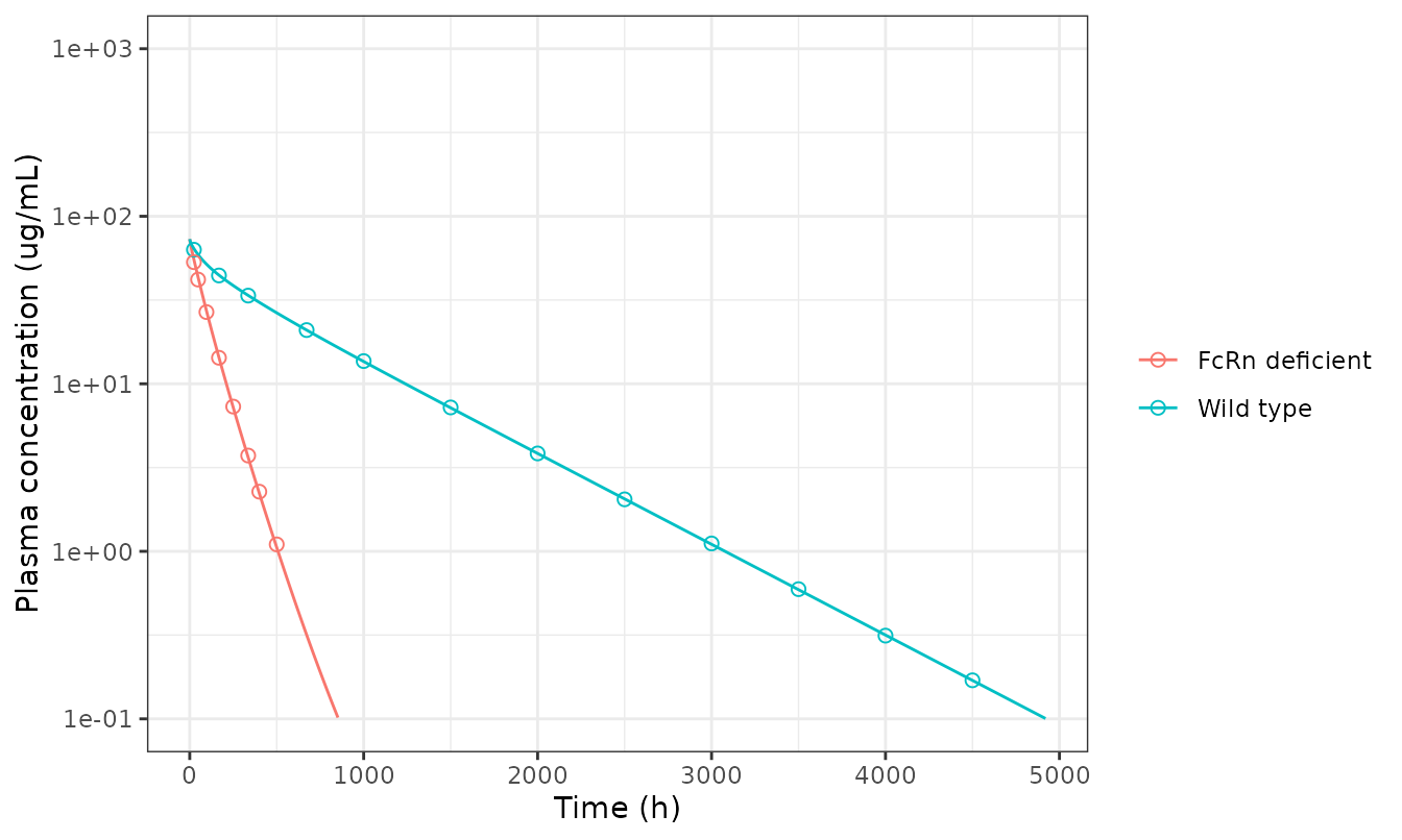
Replicates Figure 2b of Jones 2019. Lines: this model at 5 mg/kg IV. Points: the published model curves, digitised; the wild-type curve is rescaled by its constant ratio to the simulated dose.
Replicate Figures 3b and 4b: twelve clinical mAbs from their AC-SINS scores
Figures 3b (training set) and 4b (test set) give the model prediction for each human mAb, labelled with its AC-SINS score. The model uses the same FcRn affinity (700 nM) for every mAb (Methods), so the AC-SINS score is the only thing that differs between them. mAb 11 is the only subcutaneous profile. Doses are not given, so the comparison is on shape: the terminal half-life, and how constant the ratio of the published curve to the model is.
fig34 <- tibble::tribble(
  ~mab, ~acsins, ~time, ~Cc_pub,
  "mAb 01", 0, 24, 39.2,
  "mAb 01", 0, 72, 32.9,
  "mAb 01", 0, 168, 26.8,
  "mAb 01", 0, 336, 19.9,
  "mAb 01", 0, 500, 15.9,
  "mAb 01", 0, 672, 12.5,
  "mAb 01", 0, 1000, 8.34,
  "mAb 01", 0, 1500, 4.37,
  "mAb 01", 0, 2000, 2.37,
  "mAb 01", 0, 2500, 1.24,
  "mAb 01", 0, 3000, 0.671,
  "mAb 01", 0, 3500, 0.351,
  "mAb 01", 0, 4000, 0.19,
  "mAb 02", 1, 24, 80.5,
  "mAb 02", 1, 72, 67.6,
  "mAb 02", 1, 168, 54.6,
  "mAb 02", 1, 336, 40.8,
  "mAb 02", 1, 500, 32.3,
  "mAb 02", 1, 672, 25.8,
  "mAb 02", 1, 1000, 16.5,
  "mAb 02", 1, 1500, 8.66,
  "mAb 02", 1, 2000, 4.69,
  "mAb 02", 1, 2500, 2.54,
  "mAb 02", 1, 3000, 1.33,
  "mAb 02", 1, 3500, 0.721,
  "mAb 02", 1, 4000, 0.378,
  "mAb 02", 1, 4500, 0.204,
  "mAb 03", 10, 24, 28.5,
  "mAb 03", 10, 72, 15.2,
  "mAb 03", 10, 168, 8.18,
  "mAb 03", 10, 336, 4.73,
  "mAb 03", 10, 500, 3.04,
  "mAb 03", 10, 672, 1.92,
  "mAb 03", 10, 1000, 0.796,
  "mAb 03", 10, 1500, 0.206,
  "mAb 05", 4, 24, 130.0,
  "mAb 05", 4, 72, 109.0,
  "mAb 05", 4, 168, 88.8,
  "mAb 05", 4, 336, 65.9,
  "mAb 05", 4, 500, 52.8,
  "mAb 05", 4, 672, 41.6,
  "mAb 05", 4, 1000, 26.7,
  "mAb 05", 4, 1500, 14.0,
  "mAb 05", 4, 2000, 7.32,
  "mAb 05", 4, 2500, 3.83,
  "mAb 05", 4, 3000, 2.01,
  "mAb 05", 4, 3500, 1.09,
  "mAb 05", 4, 4000, 0.569,
  "mAb 05", 4, 4500, 0.298,
  "mAb 06", 1, 24, 133.0,
  "mAb 06", 1, 72, 112.0,
  "mAb 06", 1, 168, 90.5,
  "mAb 06", 1, 336, 67.9,
  "mAb 06", 1, 500, 52.7,
  "mAb 06", 1, 672, 41.6,
  "mAb 06", 1, 1000, 27.5,
  "mAb 06", 1, 1500, 14.6,
  "mAb 06", 1, 2000, 7.73,
  "mAb 06", 1, 2500, 4.08,
  "mAb 06", 1, 3000, 2.15,
  "mAb 06", 1, 3500, 1.17,
  "mAb 06", 1, 4000, 0.618,
  "mAb 06", 1, 4500, 0.337,
  "mAb 07", 17, 24, 36.8,
  "mAb 07", 17, 72, 17.0,
  "mAb 07", 17, 168, 7.22,
  "mAb 07", 17, 336, 3.55,
  "mAb 07", 17, 500, 2.25,
  "mAb 07", 17, 672, 1.35,
  "mAb 07", 17, 1000, 0.507,
  "mAb 07", 17, 1500, 0.115,
  "mAb 08", 24, 24, 17.2,
  "mAb 08", 24, 72, 7.98,
  "mAb 08", 24, 168, 3.05,
  "mAb 08", 24, 336, 1.46,
  "mAb 08", 24, 500, 0.896,
  "mAb 08", 24, 672, 0.527,
  "mAb 08", 24, 1000, 0.197,
  "mAb 11", 0, 24, 11.1,
  "mAb 11", 0, 72, 15.5,
  "mAb 11", 0, 168, 12.6,
  "mAb 11", 0, 336, 9.59,
  "mAb 11", 0, 500, 7.64,
  "mAb 11", 0, 672, 5.84,
  "mAb 11", 0, 1000, 3.82,
  "mAb 11", 0, 1500, 2.02,
  "mAb 11", 0, 2000, 1.09,
  "mAb 12", 2, 24, 77.6,
  "mAb 12", 2, 72, 67.0,
  "mAb 12", 2, 168, 53.3,
  "mAb 12", 2, 336, 39.9,
  "mAb 12", 2, 500, 32.3,
  "mAb 12", 2, 672, 25.1,
  "mAb 12", 2, 1000, 16.3,
  "mAb 12", 2, 1500, 8.66,
  "mAb 12", 2, 2000, 4.55,
  "mAb 13", 5, 24, 111.0,
  "mAb 13", 5, 72, 92.7,
  "mAb 13", 5, 168, 75.4,
  "mAb 13", 5, 336, 54.6,
  "mAb 13", 5, 500, 41.2,
  "mAb 13", 5, 672, 30.8,
  "mAb 13", 5, 1000, 17.9,
  "mAb 13", 5, 1500, 8.16,
  "mAb 13", 5, 2000, 3.82,
  "mAb 14", 1, 24, 64.1,
  "mAb 14", 1, 72, 54.0,
  "mAb 14", 1, 168, 43.5,
  "mAb 14", 1, 336, 34.1,
  "mAb 14", 1, 500, 26.2,
  "mAb 14", 1, 672, 20.5,
  "mAb 14", 1, 1000, 13.7,
  "mAb 14", 1, 1500, 7.04,
  "mAb 14", 1, 2000, 3.83,
  "mAb 23", 25, 24, 9.07,
  "mAb 23", 25, 72, 4.15,
  "mAb 23", 25, 168, 1.69,
  "mAb 23", 25, 336, 0.871,
  "mAb 23", 25, 500, 0.515,
  "mAb 23", 25, 672, 0.301,
  "mAb 23", 25, 1000, 0.113
)
mabs <- distinct(fig34, mab, acsins) |>
  mutate(
    id = row_number(),
    route = if_else(mab == "mAb 11", "SC", "IV")
  )
tgrid <- sort(unique(c(0, 0.25, 0.5, 1, 2, 4, 8, seq(12, 5000, by = 12), fig34$time)))
make_mab <- function(i) {
  bind_rows(
    data.frame(
      id = i, time = 0, amt = dose_umol, evid = 1,
      cmt = if (mabs$route[i] == "SC") "depot_sc" else "central"
    ),
    data.frame(id = i, time = tgrid, amt = 0, evid = 0, cmt = "central")
  )
}
ev_mab <- bind_rows(lapply(mabs$id, make_mab))
ev_mab$psscore <- mabs$acsins[ev_mab$id]
sim_mab <- as.data.frame(rxSolve(mod, ev_mab, keep = "psscore")) |>
  mutate(id = as.integer(id)) |>
  left_join(mabs, by = "id")
#> Warning: multi-subject simulation without without 'omega'
terminal_thalf <- function(time, conc) {
  k <- -coef(lm(log(conc) ~ time))[[2]]
  log(2) / k / 24
}
cmp34 <- inner_join(fig34, sim_mab |> select(mab, time, Cc), by = c("mab", "time")) |>
  mutate(ratio = Cc_pub / Cc)
tab34 <- cmp34 |>
  group_by(mab) |>
  arrange(time, .by_group = TRUE) |>
  summarise(
    acsins = first(acsins),
    thalf_pub_d = terminal_thalf(tail(time, 3), tail(Cc_pub, 3)),
    thalf_model_d = terminal_thalf(tail(time, 3), tail(Cc, 3)),
    ratio_cv_pct = 100 * sd(ratio) / mean(ratio),
    .groups = "drop"
  ) |>
  mutate(thalf_diff_pct = 100 * (thalf_model_d / thalf_pub_d - 1))
tab34 |>
  rename(
    "mAb" = mab, "AC-SINS" = acsins,
    "Published t1/2 (d)" = thalf_pub_d, "Model t1/2 (d)" = thalf_model_d,
    "Difference (%)" = thalf_diff_pct, "CV of ratio (%)" = ratio_cv_pct
  ) |>
knitr::kable(digits = 2, caption = "Terminal half-life over the last three digitised points of each published curve.")| mAb | AC-SINS | Published t1/2 (d) | Model t1/2 (d) | CV of ratio (%) | Difference (%) |
|---|---|---|---|---|---|
| mAb 01 | 0 | 22.89 | 23.16 | 1.33 | 1.16 |
| mAb 02 | 1 | 22.88 | 23.15 | 1.28 | 1.21 |
| mAb 03 | 10 | 10.71 | 10.74 | 1.36 | 0.32 |
| mAb 05 | 4 | 22.27 | 21.34 | 12.25 | -4.18 |
| mAb 06 | 1 | 23.20 | 23.15 | 1.67 | -0.22 |
| mAb 07 | 17 | 9.71 | 9.72 | 1.91 | 0.11 |
| mAb 08 | 24 | 9.55 | 9.57 | 4.85 | 0.26 |
| mAb 11 | 0 | 23.03 | 22.76 | 49.03 | -1.19 |
| mAb 12 | 2 | 22.63 | 22.79 | 0.93 | 0.67 |
| mAb 13 | 5 | 18.70 | 18.61 | 1.31 | -0.47 |
| mAb 14 | 1 | 22.66 | 22.85 | 1.36 | 0.83 |
| mAb 23 | 25 | 9.54 | 9.57 | 1.22 | 0.28 |
The terminal half-life matches the published curve to within 1.3% for eleven of the twelve mAbs, across AC-SINS scores from 0 to 25 (roughly 23 days down to 9.6 days). The exception is mAb 05, whose published curve decays about 4% more slowly than the model does at an AC-SINS score of 4. For mAb 11 the terminal phase matches but the absorption phase does not (hence its large ratio CV); the published curve implies a faster ka than the deposited one. Both are discussed under Assumptions and deviations.
iv <- tab34 |> filter(mab != "mAb 11")
stopifnot(
  all(abs(tab34$thalf_diff_pct) < 6),
  median(abs(tab34$thalf_diff_pct)) < 1.5,
  # Shape of every IV curve: constant ratio apart from mAb 05.
  all(iv$ratio_cv_pct[iv$mab != "mAb 05"] < 6)
)
scale34 <- cmp34 |>
  group_by(mab) |>
  summarise(s = median(ratio), .groups = "drop")
ggplot(
  sim_mab[sim_mab$time > 0 & sim_mab$Cc > 0.1, ],
  aes(time, Cc)
) +
  geom_line() +
  geom_point(
    data = fig34 |> left_join(scale34, by = "mab") |> mutate(Cc = Cc_pub / s),
    shape = 1, colour = "firebrick"
  ) +
  facet_wrap(~ paste0(mab, " (AC-SINS ", acsins, ")"), ncol = 4) +
  scale_y_log10() +
  labs(x = "Time (h)", y = "Plasma concentration (ug/mL)") +
  theme_bw()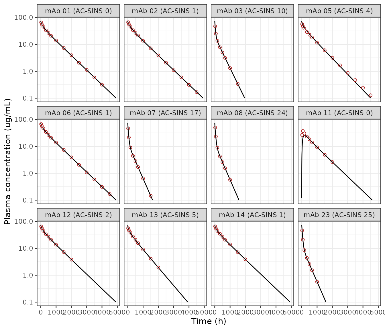
Replicates Figures 3b and 4b of Jones 2019. Lines: this model at each mAb’s AC-SINS score (5 mg/kg). Points: the published model curves, digitised and rescaled by their median ratio to the simulated dose.
PKNCA: clearance, volume and half-life across the AC-SINS range
Figure 5 plots only predicted against observed NCA parameters, and the paper prints no per-mAb numbers. The NCA below therefore compares the model’s terminal half-life with the half-life read from the published curves above. It also checks the trend stated in the Results and Discussion: “an increase in CL and Vss and a decrease in terminal T1/2 as AC-SINS score is increased”. PKNCA receives the dose in mg/kg and concentrations in mg/L, so CL is in L/h/kg and Vss in L/kg.
sim_nca <- sim_mab |>
  filter(!is.na(Cc)) |>
  select(id, time, Cc, mab)
sim_nca <- bind_rows(
  sim_nca,
  sim_nca |> distinct(id, mab) |> mutate(time = 0, Cc = 0)
) |>
  distinct(id, mab, time, .keep_all = TRUE) |>
  arrange(id, mab, time)

dose_df <- ev_mab |>
  filter(evid == 1) |>
  mutate(amt = dose_mgkg) |>
  select(id, time, amt, cmt) |>
  left_join(select(mabs, id, mab, route), by = "id")

conc_obj <- PKNCAconc(sim_nca, Cc ~ time | mab + id)
dose_obj <- PKNCAdose(
  dose_df |> mutate(route = if_else(route == "SC", "extravascular", "intravascular")),
  amt ~ time | mab + id,
  route = "route"
)
intervals <- data.frame(
  start = 0, end = Inf,
  cmax = TRUE, tmax = TRUE, aucinf.obs = TRUE, half.life = TRUE,
  cl.obs = TRUE, vss.obs = TRUE
)
nca_res <- pk.nca(PKNCAdata(conc_obj, dose_obj, intervals = intervals))

nca_wide <- as.data.frame(nca_res) |>
  filter(PPTESTCD %in% c("half.life", "cl.obs", "vss.obs")) |>
  select(mab, PPTESTCD, PPORRES) |>
  pivot_wider(names_from = PPTESTCD, values_from = PPORRES) |>
  left_join(mabs, by = "mab") |>
  arrange(acsins) |>
  mutate(
    "t1/2 (d)" = half.life / 24,
    "CL (mL/h/kg)" = 1000 * cl.obs,
    # Vss from an extravascular profile folds absorption time into the MRT,
    # so it is not a volume; blank it for the SC arm.
    "Vss (mL/kg)" = if_else(route == "SC", NA_real_, 1000 * vss.obs)
  )
nca_wide |>
  select(mab, acsins, route, "t1/2 (d)", "CL (mL/h/kg)", "Vss (mL/kg)") |>
  rename("mAb" = mab, "AC-SINS" = acsins, "Route" = route) |>
knitr::kable(digits = 3, caption = "PKNCA on the simulated profiles. For mAb 11 (SC) CL is apparent (CL/F) and Vss is not reported, because an extravascular MRT includes absorption time.")| mAb | AC-SINS | Route | t1/2 (d) | CL (mL/h/kg) | Vss (mL/kg) |
|---|---|---|---|---|---|
| mAb 01 | 0 | IV | 22.964 | 0.122 | 91.245 |
| mAb 11 | 0 | SC | 22.949 | 0.204 | NA |
| mAb 02 | 1 | IV | 22.959 | 0.122 | 91.255 |
| mAb 06 | 1 | IV | 22.959 | 0.122 | 91.255 |
| mAb 14 | 1 | IV | 22.959 | 0.122 | 91.255 |
| mAb 12 | 2 | IV | 22.895 | 0.123 | 91.371 |
| mAb 05 | 4 | IV | 21.166 | 0.137 | 94.763 |
| mAb 13 | 5 | IV | 18.640 | 0.168 | 101.702 |
| mAb 03 | 10 | IV | 10.794 | 0.538 | 159.499 |
| mAb 07 | 17 | IV | 9.731 | 0.735 | 165.140 |
| mAb 08 | 24 | IV | 9.621 | 0.764 | 164.438 |
| mAb 23 | 25 | IV | 9.617 | 0.765 | 164.400 |
published_thalf <- tab34 |>
  transmute(mab, half.life = thalf_pub_d * 24)
cmp_nca <- ncaComparisonTable(
  simulated = nca_res,
  reference = published_thalf,
  by = "mab",
  params = "half.life",
  units = c(half.life = "h"),
  tolerance_pct = 20
)
knitr::kable(
  cmp_nca,
  caption = "Terminal half-life, PKNCA on this model vs. the published model curves (Figures 3b and 4b). * differs by more than 20%."
)| NCA parameter | mab | Reference | Simulated | % diff |
|---|---|---|---|---|
| t½ (h) | mAb 01 | 549 | 551 | +0.3% |
| t½ (h) | mAb 02 | 549 | 551 | +0.4% |
| t½ (h) | mAb 03 | 257 | 259 | +0.8% |
| t½ (h) | mAb 05 | 534 | 508 | -5.0% |
| t½ (h) | mAb 06 | 557 | 551 | -1.1% |
| t½ (h) | mAb 07 | 233 | 234 | +0.2% |
| t½ (h) | mAb 08 | 229 | 231 | +0.8% |
| t½ (h) | mAb 11 | 553 | 551 | -0.4% |
| t½ (h) | mAb 12 | 543 | 549 | +1.2% |
| t½ (h) | mAb 13 | 449 | 447 | -0.3% |
| t½ (h) | mAb 14 | 544 | 551 | +1.3% |
| t½ (h) | mAb 23 | 229 | 231 | +0.8% |
No row differs by more than 20%.
iv_nca <- nca_wide |> filter(route == "IV")
typical <- iv_nca |> filter(acsins == 0)
spear <- function(x, y) suppressWarnings(cor(x, y, method = "spearman"))
c(
  rho_thalf = spear(iv_nca$acsins, iv_nca$half.life),
  rho_cl = spear(iv_nca$acsins, iv_nca$cl.obs),
  rho_vss = spear(iv_nca$acsins, iv_nca$vss.obs)
)
#> rho_thalf    rho_cl   rho_vss
#> -1.000000  1.000000  0.962963
# Deterministic model: same inputs give the same outputs on every machine.
stopifnot(
  spear(iv_nca$acsins, iv_nca$half.life) < -0.95,
  spear(iv_nca$acsins, iv_nca$cl.obs) > 0.95,
  spear(iv_nca$acsins, iv_nca$vss.obs) > 0.95,
  # Human typical-PK calibration target: terminal half-life ~20 days (Methods).
  abs(typical$half.life / 24 - 20) / 20 < 0.2
)
At an AC-SINS score of 0 the model gives CL of about 0.122 mL/h/kg, Vss of about 91.2 mL/kg and a terminal half-life of 23 days, in line with the paper’s calibration target of about 20 days for a typical human IgG1.
Sensitivity to the degradation-probability discrepancy
The deposited code and the text disagree on Prob_deg
(0.95 vs 98%; see Errata). The effect on terminal half-life:
thalf_at <- function(p) {
  s <- as.data.frame(rxSolve(mod, ev_typ, params = c(probdeg = p)))
  k <- s[s$time >= 1500 & s$time <= 3000, ]
  terminal_thalf(k$time, k$Cc)
}
pd <- c(`0.95 (deposited code)` = thalf_at(0.95), `0.98 (text, Table 1)` = thalf_at(0.98))
wt_pub <- fig2 |> filter(panel == "Wild type", time >= 1500, time <= 3000)
round(c(pd, `published Figure 2b` = terminal_thalf(wt_pub$time, wt_pub$Cc_pub)), 2)
#> 0.95 (deposited code)  0.98 (text, Table 1)   published Figure 2b
#>                 23.10                 22.65                 23.14
round(100 * (pd[[2]] / pd[[1]] - 1), 1)
#> [1] -1.9
The difference is under 2%. FcRn rescue dominates the fate of
internalised antibody, so the unrescued fraction’s exact degradation
probability matters little. The model keeps the deposited value, and
probdeg is an ini() parameter that can be
changed.
Assumptions and deviations
-
Prob_deg: 0.95 (deposited code) vs 98% (Methods, Table 1). The model uses the executable value. The published Figure 2b wild-type curve is consistent with it: its terminal half-life matches the model at 0.95 to under 1% and differs by about 2% at 0.98 (see the sensitivity section). That gap is small, so this is supporting evidence, not proof. -
Table 1 labels
kdeg_FcRn_Abin min^-1. This is a units typo: 0.062 is the per-hour value (ln 2 / 11.1 h = 0.0625 1/h), as the deposited code confirms. It is encoded per hour. -
“Other” plasma flow. Table S2 lists “Other” at 5521
mL/h and lymph node at 3670 mL/h; the deposited code uses
PLQ[Other]= 9190 mL/h (5521 + 3670 =- and represents the lymph node separately through the lymph flow. The code is followed.
-
Supplement typo in the vascular-side membrane
equation. The “VM-bound IgG due to poly-reactivity” equation in
the supplement writes
C_EXG[i, ISM]where the deposited code hasC_EXG[i, VM]. Mass balance against the VM free-antibody equation requires the code’s form, which is used. -
Subcutaneous absorption. The deposited code carries
ka = 0.26/day and F = 0.60, and the model keeps them. Methods say only
that these were “assumed” for mAb 11. The published mAb 11 curve in
Figure 4b has an earlier peak. Solving the model over a grid of ka
values reproduces its shape best at about 1.0/day (shape residual 1.6%
vs 38% at 0.26/day), so the figure was probably drawn with a faster ka
than the one deposited. Override
lkato reproduce Figure 4b(i). - mAb 05. At an AC-SINS score of 4 the model’s terminal half-life is about 4% shorter than the published curve’s. mAb 13 at a score of 5 matches to 0.3%, so one possible cause is rounding of the printed AC-SINS label (the paper prints only integer scores). The source does not settle it.
- FcRn deficiency (Figure 2b) is represented by setting total body FcRn to 1E-6 nmol. The paper does not say how its knockout arm was coded.
-
Doses of the published figures are not stated.
Comparisons are therefore on shape (terminal half-life, constancy of the
ratio). The simulations use the deposited
Dose_in_mgkg= 5. -
Endogenous IgG is clamped at 10 mg/mL in plasma
(
d/dt(C_EDG_Plasma) = 0in the deposited code), as in the source. It competes for FcRn in tissue, but its plasma pool does not respond. - Tg32 mouse arm not extracted. The deposited code is the human parameterisation. The mouse organ endothelial-cell (FcRn) fraction vector is not in any source available when this model was built; it is cited to Fan et al. 2016 (MAbs 8:848-853), which is not open access. The mouse model can be added once that source is obtained.
- No variability. The source reports neither between-subject variability nor a residual-error model; residual error is fixed at zero.