Aripiprazole lauroxil nanocrystal dispersion (Hard 2018)
Source:vignettes/articles/Hard_2018_aripiprazole_lauroxil_nanocrystal.Rmd
Hard_2018_aripiprazole_lauroxil_nanocrystal.RmdModel and source
ui <- rxode2::rxode(readModelDb("Hard_2018_aripiprazole_lauroxil_nanocrystal"))
#> ℹ parameter labels from comments will be replaced by 'label()'- Citation: Hard ML, Wehr AY, Sadler BM, Mills RJ, von Moltke L (2018). Population Pharmacokinetic Analysis and Model-Based Simulations of Aripiprazole for a 1-Day Initiation Regimen for the Long-Acting Antipsychotic Aripiprazole Lauroxil. Eur J Drug Metab Pharmacokinet 43(4):461-469. doi:10.1007/s13318-018-0488-4. All parameter estimates are from Supplementary Table S3 (Online Resource 1); the model structure is from Supplementary Fig. S1 (Online Resource 3) and the Supplementary Text (Online Resource 2). This model supersedes the earlier aripiprazole lauroxil PopPK model of Hard ML, Mills RJ, Sadler BM, Wehr AY, Weiden PJ, von Moltke L (2017) CNS Drugs 31(7):617-624, doi:10.1007/s40263-017-0447-7; see modellib(‘Hard_2017_aripiprazole_lauroxil’).
- Article: https://doi.org/10.1007/s13318-018-0488-4
- Parameter estimates: Supplementary Table S3 (Online Resource 1)
- Model schematic: Supplementary Fig. S1 (Online Resource 3)
- Model development narrative: Supplementary Text (Online Resource 2)
- Predecessor model, whose
FIM ALthis one fixes: https://doi.org/10.1007/s40263-017-0447-7 (modellib("Hard_2017_aripiprazole_lauroxil"))
Aripiprazole lauroxil (AL) is an intramuscular extended-release prodrug of aripiprazole. Starting AL normally requires 21 days of daily oral aripiprazole supplementation. To replace that, Alkermes developed a nanocrystal milled dispersion of the same prodrug (ALNCD), whose smaller particles dissolve faster; a single ALNCD injection plus a single 30 mg oral aripiprazole dose is the 1-day initiation regimen.
This model therefore has to describe three chemically distinct inputs of one analyte, and that is what makes it worth having in the library.
Structure
Supplementary Fig. S1 draws three inputs into a single aripiprazole
central compartment that exchanges with one peripheral compartment and
is cleared by CL/F:
| Input | Mechanism | Encoded as |
|---|---|---|
| Oral aripiprazole | first order at Ka
|
depot, f(depot) = 1 (the reference
route) |
| Aripiprazole lauroxil IM | zero order over D AL, after a lag
ALAG AL
|
lagged modelled-duration input straight into
central
|
| ALNCD IM | double Weibull dissolution |
depot2 (slow) + depot3 (fast), emptying at
Weibull hazards |
cat(paste(rxode2::modelExtract(ui), collapse = "\n"))
#> cl <- exp(lcl + etalcl)
#> vc <- exp(lvc + etalvc) * (WT/70)^e_wt_vc
#> vp <- exp(lvp + etalvp)
#> q <- exp(lq + etalq)
#> ka <- exp(lka + etalka)
#> d1 <- exp(ld1 + etald1)
#> tlag <- exp(ltlag + etaltlag)
#> c0 <- exp(lc0 + etalc0)
#> fdepot <- exp(lfdepot)
#> fdepot_im <- exp(lfdepot_im + etalfdepot_im)
#> fdepot_ncd <- exp(lfdepot_ncd)
#> wa1 <- exp(lwa1 + etalwa1)
#> wa2 <- exp(lwa2 + etalwa2)
#> wb1i <- wb1 * exp(etawb1)
#> wb2i <- wb2 * exp(etawb2)
#> fracw <- expit(logitfrac * exp(etalogitfrac), 0, 1)
#> kel <- cl/vc
#> k12 <- q/vc
#> k21 <- q/vp
#> h1 <- min((wb1i/wa1) * (tad0(depot2)/wa1)^(wb1i - 1), 50/wa1)
#> h2 <- min((wb2i/wa2) * (tad0(depot3)/wa2)^(wb2i - 1), 50/wa2)
#> d/dt(depot) <- -ka * depot
#> d/dt(depot2) <- -h1 * depot2
#> d/dt(depot3) <- -h2 * depot3
#> d/dt(central) <- ka * depot + h1 * depot2 + h2 * depot3 - kel * central - k12 * central + k21 * peripheral1
#> d/dt(peripheral1) <- k12 * central - k21 * peripheral1
#> central(0) <- c0 * vc/1000
#> f(depot) <- fdepot
#> f(depot2) <- fdepot_im * fdepot_ncd * fracw
#> f(depot3) <- fdepot_im * fdepot_ncd * (1 - fracw)
#> f(central) <- fdepot_im
#> dur(central) <- d1
#> alag(central) <- tlag
#> Cc <- 1000 * central/vc
#> propSdStudy <- propSdStdyA105 * STUDY_A105 + propSdStdyAlncd * (1 - STUDY_A105)
Consequences for a user’s data set:
-
AL doses use
cmt = "central"withrate = -2, so rxode2 uses the modelled durationdur(central) <- d1. Withoutrate = -2rxode2 silently delivers a bolus. The amount is the aripiprazole-equivalent dose, not the AL dose: the paper’s mapping (Sect. 2.1.2) is 110 / 221 / 441 / 662 / 882 / 1064 mg AL or ALNCD = 75 / 150 / 300 / 450 / 600 / 724 mg aripiprazole. -
ALNCD doses are entered as two
records carrying the same
amt, one intodepot2and one intodepot3. Thef()factors apply the bioavailability and split the dose between the two Weibull pathways, so the total delivered is one dose, not two. -
Oral aripiprazole doses use
cmt = "depot". -
WT(kg) andSTUDY_A105(1 for study ALK9072-A105, else 0) are required on every record.
The double Weibull
The fraction of an ALNCD injection released by time
t after the injection is a two-component Weibull
mixture,
with MDT1 = 596 h (24.8 days) the slow component and
MDT2 = 76.7 h (3.2 days) the fast one. Encoding it as two
depots emptying at the corresponding Weibull hazards is the same
parameterisation nlmixr2lib::addWeibullAbs() uses.
The paper never writes this equation down, and it never says
what p is. Supplementary Table S3 reports
FRAC = 2.02, which cannot be a bare fraction. The transform
is therefore inferred, and the inference is validated below against an
independently published study. See Assumptions and
deviations.
Population
pop <- ui$population
str(pop, max.level = 1)
#> List of 14
#>  $ species       : chr "human"
#>  $ n_subjects    : num 343
#>  $ n_studies     : num 4
#>  $ age_range     : chr "adults"
#>  $ age_median    : chr "mean 45.2 years (SD 10.8)"
#>  $ weight_range  : chr "not reported"
#>  $ weight_median : chr "mean 89.1 kg (SD 17.9)"
#>  $ sex_female_pct: num 27
#>  $ race_ethnicity: Named num [1:3] 78 21 1
#>   ..- attr(*, "names")= chr [1:3] "Black" "White" "Other"
#>  $ disease_state : chr "schizophrenia or schizoaffective disorder, stable on a first-line antipsychotic other than aripiprazole"
#>  $ dose_range    : chr "aripiprazole lauroxil 441-1064 mg IM and nanocrystal dispersion 110-662 mg IM (modelled as aripiprazole equival"| __truncated__
#>  $ regions       : chr "USA"
#>  $ cyp2d6        : chr "extensive and intermediate metabolizers plus inconclusive phenotypes; poor metabolizers were absent (excluded f"| __truncated__
#>  $ notes         : chr "12,768 plasma aripiprazole concentrations (351 [3%] below the lower limit of quantitation of 1 ng/mL, handled b"| __truncated__
12,768 plasma aripiprazole concentrations (351 [3%] below the 1 ng/mL limit of quantitation, retained by the M3 method) from 343 patients with schizophrenia or schizoaffective disorder across four phase I studies (Table 1 and Supplementary Table S1):
| Study | Code | n | What it contributed |
|---|---|---|---|
| 1 | ALK9072-B101 | 41 | single ascending ALNCD doses, gluteal |
| 2 | ALK9072-B102 | 161 | ALNCD + 30 mg oral + AL 441/882 mg, vs the 21-day oral regimen |
| 3 | ALK9072-B103 | 47 | ALNCD deltoid vs gluteal |
| 4 | ALK9072-A105 | 94 | AL alone, q4wk / q6wk / q8wk |
Mean age 45.2 years, 73% men, 78% Black or African American, mean weight 89.1 kg. CYP2D6 poor metabolizers were excluded from studies 1-3 and absent from the data set, so the model carries no CYP2D6 term and the paper states explicitly that its findings do not apply to poor metabolizers.
Source trace
Every ini() entry in
inst/modeldb/specificDrugs/Hard_2018_aripiprazole_lauroxil_nanocrystal.R
carries an in-file comment pointing at its source location. They are
collected here. Every value is from Supplementary Table S3 unless
noted.
| Parameter | Value | Source location |
|---|---|---|
lcl (CL/F) |
1.98 L/h | row CL/F (L/h), %RSE 2.54 |
lvc (VC/F) |
327 L at 70 kg | row VC/F (L), %RSE 4.51 |
lvp (VP/F) |
1720 L | row VP/F (L), %RSE 13.9 |
lq (Q/F) |
0.102 L/h | row Q/F (L/h), %RSE 10.9 |
lka (Ka oral) |
0.47 1/h | row Ka PO ARI (h-1), %RSE 14.2 |
ld1 (D AL) |
934 h | row D AL (h), %RSE 3.86 |
ltlag (ALAG AL) |
106 h | row ALAG AL (h), %RSE 7.85 |
lwa1 (MDT1) |
596 h | row MDT1 (h), %RSE 3.29 |
wb1 (GAM1) |
2.2 | row GAM1, %RSE 2.85 |
lwa2 (MDT2) |
76.7 h | row MDT2 (h), %RSE 4.47 |
wb2 (GAM2) |
2.09 | row GAM2, %RSE 2.36 |
logitfrac (FRAC) |
2.02 | row FRAC, %RSE 3.88 |
lfdepot (FPO) |
1, fixed | row FPO ARI, footnote a “Fixed at 1.00” |
lfdepot_im (FIM AL) |
0.571, fixed | row FIM AL, footnote b “Fixed at 57.1% from previous
analysis” |
lfdepot_ncd (FIM ALNCD) |
1.12 | row FIM ALNCD, footnote c “ALNCD F estimated relative
to AL” |
lc0 (ARI(0)) |
0.378 ng/mL | row ARI(0) (ng/mL), %RSE 14.8 |
e_wt_vc |
1, fixed | row Weight ON VC/F, footnotes a and f |
| weight centering (70 kg) | 70 kg | Sect. 2.1.2, “fixed allometric exponents of 0.75 and 1 … scaled to 70 kg” |
| IIV variances (14 etas) | see model file | “Interindividual variability” block |
propSdStdyAlncd |
sqrt(0.0359) | row sigma2 prop Studies 1, 2, and 3
|
propSdStdyA105 |
sqrt(0.0207) | row sigma2 prop Study 4
|
| Model topology | n/a | Supplementary Fig. S1 |
| Double Weibull for ALNCD | n/a | Supplementary Fig. S1 and Sect. 3.1.2 |
| Zero-order AL input with lag | n/a | Sect. 3.1.2 |
The IIV column is a variance
Supplementary Table S3’s “Interindividual variability / Point
Estimate” column holds omega^2. Footnote e
gives CV = sqrt(exp(omega^2) - 1) * 100 for the rows it
flags; the two unflagged rows use the small-variance approximation
sqrt(omega^2) that Online Resource 2 describes for
variances below 0.15. Every published CV is reproduced below from the
encoded variances, which is what confirms the variance reading.
published_cv <- c(
  etalcl = 84.5, etalvc = 52.0, etalwa1 = 46.7, etawb1 = 76.5,
  etalwa2 = 56.1, etawb2 = 35.9, etalogitfrac = 129, etalvp = 99.3,
  etalq = 353, etalka = 325, etald1 = 38.3, etaltlag = 120,
  etalfdepot_im = 81.1, etalc0 = 870
)

etas <- ui$iniDf |>
  dplyr::filter(!is.na(neta1), neta1 == neta2) |>
  dplyr::transmute(
    eta = name,
    omega2 = est,
    `CV% via sqrt(exp(w2)-1)` = round(100 * sqrt(exp(est) - 1), 1),
    `CV% via sqrt(w2)` = round(100 * sqrt(est), 1),
    `Published CV%` = published_cv[name]
  )
knitr::kable(
  etas,
  digits = 3,
  caption = "Supplementary Table S3's IIV column reproduced from the encoded variances. Every row matches one of the two formulae the table itself uses; GAM2 (35.9%) and D AL (38.3%) are the two rows that use the small-variance approximation."
)| eta | omega2 | CV% via sqrt(exp(w2)-1) | CV% via sqrt(w2) | Published CV% |
|---|---|---|---|---|
| etalcl | 0.539 | 84.5 | 73.4 | 84.5 |
| etalvc | 0.239 | 52.0 | 48.9 | 52.0 |
| etalwa1 | 0.197 | 46.7 | 44.4 | 46.7 |
| etawb1 | 0.461 | 76.5 | 67.9 | 76.5 |
| etalwa2 | 0.274 | 56.1 | 52.3 | 56.1 |
| etawb2 | 0.129 | 37.1 | 35.9 | 35.9 |
| etalogitfrac | 0.978 | 128.8 | 98.9 | 129.0 |
| etalvp | 0.686 | 99.3 | 82.8 | 99.3 |
| etalq | 2.600 | 353.0 | 161.2 | 353.0 |
| etalka | 2.450 | 325.4 | 156.5 | 325.0 |
| etald1 | 0.147 | 39.8 | 38.3 | 38.3 |
| etaltlag | 0.895 | 120.3 | 94.6 | 120.0 |
| etalfdepot_im | 0.505 | 81.1 | 71.1 | 81.1 |
| etalc0 | 4.340 | 870.1 | 208.3 | 870.0 |
# Arithmetic on fixed numbers -- no simulation -- so the bound is tight by
# construction and 1 CV point is pure rounding headroom.
matched <- pmin(
  abs(etas$`CV% via sqrt(exp(w2)-1)` - etas$`Published CV%`),
  abs(etas$`CV% via sqrt(w2)` - etas$`Published CV%`)
)
stopifnot(nrow(etas) == 14L, !anyNA(matched), all(matched < 1.0))
Structural checks
Deterministic: these solve the typical-value model
(zeroRe()) and compare against closed-form identities, so
the tolerances are numerical rather than statistical and are correctly
tight.
mod_tv <- rxode2::zeroRe(ui)
#> Warning: No sigma parameters in the model
th <- ui$theta

cl_typ <- exp(th[["lcl"]])
vc70 <- exp(th[["lvc"]])
vp_typ <- exp(th[["lvp"]])
q_typ <- exp(th[["lq"]])
d1_typ <- exp(th[["ld1"]])
tlag_typ <- exp(th[["ltlag"]])
c0_typ <- exp(th[["lc0"]])
fim_typ <- exp(th[["lfdepot_im"]])
fncd_typ <- fim_typ * exp(th[["lfdepot_ncd"]])
frac_typ <- 1 / (1 + exp(-th[["logitfrac"]]))

# Aripiprazole-equivalent dose for each AL / ALNCD strength (Sect. 2.1.2).
eq_dose <- c(`110` = 75, `221` = 150, `441` = 300, `662` = 450, `882` = 600, `1064` = 724)

solve_tv <- function(events) {
  suppressWarnings(rxode2::rxSolve(mod_tv, events, addDosing = FALSE)) |>
    as.data.frame() |>
    dplyr::filter(!is.na(Cc))
}
trap <- function(tm, cc) sum(diff(tm) * (head(cc, -1) + tail(cc, -1)) / 2)

# Observation grid: dense over the first two days so the oral peak is resolved,
# coarse afterwards so the 300-day AL and ALNCD tails are still covered. A grid
# that misses Tmax understates AUC and would make the mass-balance identity
# below look violated when it is not.
tv_events <- function(doses, horizon_h) {
  grid <- sort(unique(c(seq(0, 48, by = 0.25), seq(0, horizon_h, by = 6))))
  obs <- data.frame(
    id = 1L, time = grid, amt = NA_real_, evid = 0L, cmt = "central",
    rate = NA_real_, WT = 70, STUDY_A105 = 0
  )
  dplyr::arrange(dplyr::bind_rows(doses, obs), time, dplyr::desc(evid))
}
al_dose <- function(times_h, amt) {
  data.frame(
    id = 1L, time = times_h, amt = amt, evid = 1L, cmt = "central",
    rate = -2, WT = 70, STUDY_A105 = 0
  )
}
ncd_dose <- function(times_h, amt) {
  do.call(rbind, lapply(c("depot2", "depot3"), function(cm) {
    data.frame(
      id = 1L, time = times_h, amt = amt, evid = 1L, cmt = cm,
      rate = NA_real_, WT = 70, STUDY_A105 = 0
    )
  }))
}
po_dose <- function(times_h, amt) {
  data.frame(
    id = 1L, time = times_h, amt = amt, evid = 1L, cmt = "depot",
    rate = NA_real_, WT = 70, STUDY_A105 = 0
  )
}
Mass balance: CL/F * AUC(0-inf) == F * Dose + A0
The one invariant a mis-transcribed clearance, dose, bioavailability or unit conversion cannot survive. It is blind to how the dose is spread in time, so it runs on all three input routes – including the double Weibull, where it is also the check that the two pathways together deliver exactly one dose.
horizon <- 250000 # h; long enough for the ~500-day beta phase to be exhausted
baseline_mg <- c0_typ * vc70 / 1000

mb <- tibble::tibble(
  Route = c(
    "Oral, single 15 mg",
    "AL IM, single 441 mg (300 mg equivalent)",
    "ALNCD IM, single 662 mg (450 mg equivalent)"
  ),
  Recovered = c(
    cl_typ * trap(solve_tv(tv_events(po_dose(0, 15), horizon))$time,
                  solve_tv(tv_events(po_dose(0, 15), horizon))$Cc) / 1000,
    cl_typ * trap(solve_tv(tv_events(al_dose(0, eq_dose[["441"]]), horizon))$time,
                  solve_tv(tv_events(al_dose(0, eq_dose[["441"]]), horizon))$Cc) / 1000,
    cl_typ * trap(solve_tv(tv_events(ncd_dose(0, eq_dose[["662"]]), horizon))$time,
                  solve_tv(tv_events(ncd_dose(0, eq_dose[["662"]]), horizon))$Cc) / 1000
  ),
  Expected = c(
    1 * 15 + baseline_mg,
    fim_typ * eq_dose[["441"]] + baseline_mg,
    fncd_typ * eq_dose[["662"]] + baseline_mg
  )
) |>
  dplyr::mutate(Ratio = Recovered / Expected) |>
  dplyr::rename(
    "Recovered CL/F * AUCinf (mg)" = Recovered,
    "Expected F * Dose + A0 (mg)" = Expected
  )
#> ℹ omega/sigma items treated as zero: 'etalcl', 'etalvc', 'etalwa1', 'etawb1', 'etalwa2', 'etawb2', 'etalogitfrac', 'etalvp', 'etalq', 'etalka', 'etald1', 'etaltlag', 'etalfdepot_im', 'etalc0'
#> ℹ omega/sigma items treated as zero: 'etalcl', 'etalvc', 'etalwa1', 'etawb1', 'etalwa2', 'etawb2', 'etalogitfrac', 'etalvp', 'etalq', 'etalka', 'etald1', 'etaltlag', 'etalfdepot_im', 'etalc0'
#> ℹ omega/sigma items treated as zero: 'etalcl', 'etalvc', 'etalwa1', 'etawb1', 'etalwa2', 'etawb2', 'etalogitfrac', 'etalvp', 'etalq', 'etalka', 'etald1', 'etaltlag', 'etalfdepot_im', 'etalc0'
#> ℹ omega/sigma items treated as zero: 'etalcl', 'etalvc', 'etalwa1', 'etawb1', 'etalwa2', 'etawb2', 'etalogitfrac', 'etalvp', 'etalq', 'etalka', 'etald1', 'etaltlag', 'etalfdepot_im', 'etalc0'
#> ℹ omega/sigma items treated as zero: 'etalcl', 'etalvc', 'etalwa1', 'etawb1', 'etalwa2', 'etawb2', 'etalogitfrac', 'etalvp', 'etalq', 'etalka', 'etald1', 'etaltlag', 'etalfdepot_im', 'etalc0'
#> ℹ omega/sigma items treated as zero: 'etalcl', 'etalvc', 'etalwa1', 'etawb1', 'etalwa2', 'etawb2', 'etalogitfrac', 'etalvp', 'etalq', 'etalka', 'etald1', 'etaltlag', 'etalfdepot_im', 'etalc0'
knitr::kable(mb, digits = c(0, 3, 3, 5))| Route | Recovered CL/F * AUCinf (mg) | Expected F * Dose + A0 (mg) | Ratio |
|---|---|---|---|
| Oral, single 15 mg | 15.125 | 15.124 | 1.00007 |
| AL IM, single 441 mg (300 mg equivalent) | 171.424 | 171.424 | 1.00000 |
| ALNCD IM, single 662 mg (450 mg equivalent) | 287.901 | 287.908 | 0.99998 |
The AL zero-order input window
A single AL injection must peak exactly at ALAG + D AL,
the moment the zero-order input stops, and nothing may enter
central during the lag.
sd <- solve_tv(dplyr::arrange(
  dplyr::bind_rows(
    al_dose(0, eq_dose[["441"]]),
    data.frame(
      id = 1L, time = seq(0, 3000, by = 1), amt = NA_real_, evid = 0L,
      cmt = "central", rate = NA_real_, WT = 70, STUDY_A105 = 0
    )
  ),
  time, dplyr::desc(evid)
))
#> ℹ omega/sigma items treated as zero: 'etalcl', 'etalvc', 'etalwa1', 'etawb1', 'etalwa2', 'etawb2', 'etalogitfrac', 'etalvp', 'etalq', 'etalka', 'etald1', 'etaltlag', 'etalfdepot_im', 'etalc0'

tmax_al <- sd$time[which.max(sd$Cc)]
pre_lag <- sd$Cc[sd$time == floor(tlag_typ) - 7]
post_lag <- sd$Cc[sd$time == ceiling(tlag_typ) + 7]

knitr::kable(
  tibble::tibble(
    Quantity = c(
      "Tmax after a single AL injection (h)", "ALAG + D AL (h)",
      "Cc 7 h before the lag ends (ng/mL)", "Cc 7 h after the lag ends (ng/mL)"
    ),
    Value = c(tmax_al, tlag_typ + d1_typ, pre_lag, post_lag)
  ),
  digits = 3
)| Quantity | Value |
|---|---|
| Tmax after a single AL injection (h) | 1040.000 |
| ALAG + D AL (h) | 1040.000 |
| Cc 7 h before the lag ends (ng/mL) | 0.203 |
| Cc 7 h after the lag ends (ng/mL) | 4.024 |
The Weibull split really is expit(FRAC)
The encoded model must deliver expit(2.02) = 88.3% of an
ALNCD injection through the slow (MDT1) pathway
and the rest through the fast one. This reads the split back out of the
solved depots rather than trusting the ini() line.
depots <- suppressWarnings(rxode2::rxSolve(
  mod_tv,
  dplyr::arrange(
    dplyr::bind_rows(
      ncd_dose(0, eq_dose[["662"]]),
      data.frame(
        id = 1L, time = c(0, 1e-6), amt = NA_real_, evid = 0L, cmt = "central",
        rate = NA_real_, WT = 70, STUDY_A105 = 0
      )
    ),
    time, dplyr::desc(evid)
  ),
  addDosing = FALSE
)) |>
  as.data.frame() |>
  dplyr::slice_max(time, n = 1)
#> ℹ omega/sigma items treated as zero: 'etalcl', 'etalvc', 'etalwa1', 'etawb1', 'etalwa2', 'etawb2', 'etalogitfrac', 'etalvp', 'etalq', 'etalka', 'etald1', 'etaltlag', 'etalfdepot_im', 'etalc0'

split <- tibble::tibble(
  Quantity = c(
    "Slow (MDT1) depot at t = 0 (mg)",
    "Fast (MDT2) depot at t = 0 (mg)",
    "Slow share of the delivered dose",
    "expit(FRAC)",
    "Total delivered (mg)",
    "FIM ALNCD * FIM AL * dose (mg)"
  ),
  Value = c(
    depots$depot2, depots$depot3,
    depots$depot2 / (depots$depot2 + depots$depot3),
    frac_typ,
    depots$depot2 + depots$depot3,
    fncd_typ * eq_dose[["662"]]
  )
)
knitr::kable(split, digits = 4)| Quantity | Value |
|---|---|
| Slow (MDT1) depot at t = 0 (mg) | 254.0790 |
| Fast (MDT2) depot at t = 0 (mg) | 33.7050 |
| Slow share of the delivered dose | 0.8829 |
| expit(FRAC) | 0.8829 |
| Total delivered (mg) | 287.7840 |
| FIM ALNCD * FIM AL * dose (mg) | 287.7840 |
The weight covariate moves volume, not exposure
WT enters only Vc/F, with the exponent
fixed at 1. Exposure is clearance-determined, so AUC must be
exactly invariant to weight on every route. What
happens to Cmax is route-dependent, and the contrast is a
useful structural check in its own right:
- After oral dosing the peak is reached while
distribution still matters, so
Cmaxtracks1/Vcand its 120 kg : 70 kg ratio sits just above the instantaneous-bolus limit of 70/120. - After an AL injection the zero-order input runs for
934 h, far longer than the 4.5-day distribution half-life, so the
profile plateaus near
input rate / CL– a quantity that does not containVcat all.Cmaxis therefore almost weight-independent.
auc_cmax_at <- function(wt, doses) {
  ev <- tv_events(doses, 30000)
  ev$WT <- wt
  s <- solve_tv(ev)
  c(auc = trap(s$time, s$Cc), cmax = max(s$Cc))
}
routes <- list(
  `AL IM, 441 mg` = al_dose(0, eq_dose[["441"]]),
  `Oral, 15 mg` = po_dose(0, 15)
)
cov_chk <- dplyr::bind_rows(lapply(names(routes), function(nm) {
  a <- auc_cmax_at(70, routes[[nm]])
  b <- auc_cmax_at(120, routes[[nm]])
  tibble::tibble(
    Route = nm,
    `AUCinf ratio 120:70 kg` = b[["auc"]] / a[["auc"]],
    `Cmax ratio 120:70 kg` = b[["cmax"]] / a[["cmax"]]
  )
}))
#> ℹ omega/sigma items treated as zero: 'etalcl', 'etalvc', 'etalwa1', 'etawb1', 'etalwa2', 'etawb2', 'etalogitfrac', 'etalvp', 'etalq', 'etalka', 'etald1', 'etaltlag', 'etalfdepot_im', 'etalc0'
#> ℹ omega/sigma items treated as zero: 'etalcl', 'etalvc', 'etalwa1', 'etawb1', 'etalwa2', 'etawb2', 'etalogitfrac', 'etalvp', 'etalq', 'etalka', 'etald1', 'etaltlag', 'etalfdepot_im', 'etalc0'
#> ℹ omega/sigma items treated as zero: 'etalcl', 'etalvc', 'etalwa1', 'etawb1', 'etalwa2', 'etawb2', 'etalogitfrac', 'etalvp', 'etalq', 'etalka', 'etald1', 'etaltlag', 'etalfdepot_im', 'etalc0'
#> ℹ omega/sigma items treated as zero: 'etalcl', 'etalvc', 'etalwa1', 'etawb1', 'etalwa2', 'etawb2', 'etalogitfrac', 'etalvp', 'etalq', 'etalka', 'etald1', 'etaltlag', 'etalfdepot_im', 'etalc0'
cov_chk$`70/120` <- 70 / 120
knitr::kable(cov_chk, digits = 4)| Route | AUCinf ratio 120:70 kg | Cmax ratio 120:70 kg | 70/120 |
|---|---|---|---|
| AL IM, 441 mg | 1.0004 | 0.9708 | 0.5833 |
| Oral, 15 mg | 1.0057 | 0.5989 | 0.5833 |
stopifnot(
  # AUC invariance is an identity: both sides share CL/F and the dose.
  all(abs(cov_chk$`AUCinf ratio 120:70 kg` - 1) < 0.01),
  # Oral Cmax is volume-dominated and must sit just above the bolus limit.
  cov_chk$`Cmax ratio 120:70 kg`[2] > 70 / 120,
  cov_chk$`Cmax ratio 120:70 kg`[2] < 70 / 120 + 0.05,
  # AL Cmax is plateau-dominated and must be nearly weight-free.
  cov_chk$`Cmax ratio 120:70 kg`[1] > 0.9
)
Validating the double Weibull against study ALK9072-B103
This is the load-bearing check of the vignette, because
FRAC = 2.02 is the one value in the model whose meaning had
to be inferred.
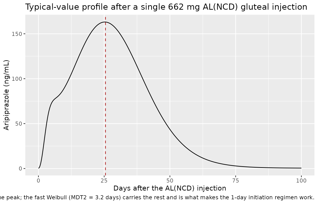
Study 3 of this analysis, ALK9072-B103, was published separately with a full non-compartmental analysis of ALNCD given alone (Hard ML, Wehr A, von Moltke L, Du Y, Farwick S, Walling D, Sonnenberg J. Ther Adv Psychopharmacol 2019;9:2045125319859964, https://doi.org/10.1177/2045125319859964; the 662 mg ALNCD dose is confirmed in Hard ML et al., J Clin Psychopharmacol 2018;38(5):435-441, https://doi.org/10.1097/JCP.0000000000000921, which states that the clinical studies used “a 662-mg dose of ALNCD”). Its gluteal arm is the reference injection site of this model, and its numbers played no part in choosing the transform, so it is a genuine out-of-sample test of the ALNCD input function.
Published, gluteal arm, n = 24:
| Parameter | Published |
|---|---|
| Cmax | mean 175.0 ng/mL (SD 85.0, 48.6% CV) |
| tmax | median 25.5 days (range 10.0, 41.0) |
| AUClast | mean 6070.2 day*ng/mL (35.8% CV) |
| AUCinf | mean 6437.2 day*ng/mL (34.4% CV) |
| t1/2 | mean 15.2 days (41.5% CV) |
Typical-value profile
# ALK9072-B103 PK sampling days.
b103_days <- c(1, 2, 3, 5, 8, 10, 12, 17, 19, 21, 23, 25, 27, 30, 33, 36, 43,
               57, 71, 80, 85)
b103_times <- (b103_days - 1) * 24
b103_wt <- 86.6 # study 3 mean weight, Table 1

ev_b103_tv <- dplyr::arrange(
  dplyr::bind_rows(
    ncd_dose(0, eq_dose[["662"]]),
    data.frame(
      id = 1L, time = seq(0, 100 * 24, by = 2), amt = NA_real_, evid = 0L,
      cmt = "central", rate = NA_real_, WT = 70, STUDY_A105 = 0
    )
  ),
  time, dplyr::desc(evid)
)
ev_b103_tv$WT <- b103_wt
tv_b103 <- solve_tv(ev_b103_tv)
#> ℹ omega/sigma items treated as zero: 'etalcl', 'etalvc', 'etalwa1', 'etawb1', 'etalwa2', 'etawb2', 'etalogitfrac', 'etalvp', 'etalq', 'etalka', 'etald1', 'etaltlag', 'etalfdepot_im', 'etalc0'

b103_tv <- tibble::tibble(
  Quantity = c("Cmax (ng/mL)", "tmax (days)"),
  `Typical value` = c(max(tv_b103$Cc), tv_b103$time[which.max(tv_b103$Cc)] / 24),
  `Published` = c(175.0, 25.5),
  `Published median-scaled` = c(175.0 / sqrt(1 + 0.486^2), 25.5)
)
knitr::kable(
  b103_tv,
  digits = 2,
  caption = "Typical-value AL_NCD profile against the published study B103 gluteal arm. The published Cmax is an arithmetic mean over a 48.6% CV cohort, so the median it implies (mean / sqrt(1 + CV^2)) is the fairer comparator for a typical-value prediction; tmax is already published as a median."
)| Quantity | Typical value | Published | Published median-scaled |
|---|---|---|---|
| Cmax (ng/mL) | 163.11 | 175.0 | 157.4 |
| tmax (days) | 25.25 | 25.5 | 25.5 |
# tmax is the statistic that actually discriminates the candidate transforms.
# Every other reading of FRAC that was tried (FRAC/(1+FRAC) = 0.669,
# 1/FRAC = 0.495, 1/(1+FRAC) = 0.331) puts the typical-value tmax near 5 days
# rather than near 25; see "Assumptions and deviations". The bound below is
# generous against the published median's own precision -- n = 24 on an
# irregular sampling grid whose observed range was 10 to 41 days -- and still
# excludes every alternative transform by a factor of four.
stopifnot(
  abs(b103_tv$`Typical value`[2] - 25.5) < 6,
  abs(b103_tv$`Typical value`[1] / b103_tv$`Published median-scaled`[1] - 1) < 0.25
)
ggplot(tv_b103, aes(time / 24, Cc)) +
  geom_line() +
  geom_vline(xintercept = 25.5, linetype = 2, colour = "firebrick") +
  labs(
    x = "Days after the AL(NCD) injection", y = "Aripiprazole (ng/mL)",
    title = "Typical-value profile after a single 662 mg AL(NCD) gluteal injection",
    caption = paste(
      "Dashed red line = the published median tmax of 25.5 days in the gluteal",
      "arm of study ALK9072-B103. The slow Weibull (MDT1 = 24.8 days) carries",
      "88% of the dose and sets the peak; the fast Weibull (MDT2 = 3.2 days)",
      "carries the rest and is what makes the 1-day initiation regimen work."
    )
  )
Cohort non-compartmental analysis
set.seed(20260918)
rxode2::rxSetSeed(20260918)
n_b103 <- 200

# Study 3 weight, Table 1: mean 86.6 kg (SD 15.6); clipped to a plausible range.
wt_b103 <- pmin(pmax(stats::rnorm(n_b103, 86.6, 15.6), 45), 145)

ev_b103 <- dplyr::arrange(
  dplyr::bind_rows(
    do.call(rbind, lapply(c("depot2", "depot3"), function(cm) {
      data.frame(
        id = seq_len(n_b103), time = 0, amt = eq_dose[["662"]], evid = 1L,
        cmt = cm, WT = wt_b103, STUDY_A105 = 0
      )
    })),
    data.frame(
      id = rep(seq_len(n_b103), each = length(b103_times)),
      time = rep(b103_times, times = n_b103),
      amt = NA_real_, evid = 0L, cmt = "central",
      WT = rep(wt_b103, each = length(b103_times)), STUDY_A105 = 0
    )
  ),
  id, time, dplyr::desc(evid)
)

sim_b103 <- suppressWarnings(rxode2::rxSolve(ui, ev_b103, addDosing = FALSE)) |>
  as.data.frame() |>
  dplyr::filter(!is.na(Cc)) |>
  dplyr::mutate(time_d = time / 24)

# Extreme eta draws can decay into solver round-off in the far tail. Assert on
# the magnitude of any negative value -- orders of magnitude below the cohort
# median, so a genuinely negative prediction still goes red -- then clamp.
stopifnot(min(c(0, sim_b103$Cc)) > -1e-6)
sim_b103$Cc <- pmax(sim_b103$Cc, 0)
The PKNCA input is filtered on !is.na(Cc) only. Day 1 of
the study is time zero, so the time-zero record the AUC
interval needs is already present and must not be filtered out.
conc_obj <- PKNCA::PKNCAconc(
  dplyr::select(sim_b103, id, time_d, Cc),
  Cc ~ time_d | id, concu = "ng/mL", timeu = "day"
)
dose_obj <- PKNCA::PKNCAdose(
  data.frame(id = seq_len(n_b103), time_d = 0, amt = eq_dose[["662"]]),
  amt ~ time_d | id, doseu = "mg"
)
nca_b103 <- suppressWarnings(PKNCA::pk.nca(PKNCA::PKNCAdata(
  conc_obj, dose_obj,
  intervals = data.frame(
    start = 0, end = Inf,
    cmax = TRUE, tmax = TRUE, auclast = TRUE, aucinf.obs = TRUE,
    half.life = TRUE
  )
)))
published_b103 <- data.frame(
  cmax = 175.0, tmax = 25.5, auclast = 6070.2, aucinf.obs = 6437.2,
  half.life = 15.2
)

cmp_b103 <- nlmixr2lib::ncaComparisonTable(
  simulated = nca_b103,
  reference = published_b103,
  units = c(cmax = "ng/mL", tmax = "day", auclast = "day*ng/mL",
            aucinf.obs = "day*ng/mL", half.life = "day"),
  tolerance_pct = 20
)
knitr::kable(
  cmp_b103,
  align = c("l", "r", "r", "r"),
  caption = paste(
    "Simulated 200-subject cohort (pooled by median) against the published",
    "gluteal arm of study ALK9072-B103 (arithmetic means, except tmax which is",
    "a median).", attr(cmp_b103, "footnote")
  )
)| NCA parameter | Reference | Simulated | % diff |
|---|---|---|---|
| Cmax (ng/mL) | 175 | 175 | +0.0% |
| Tmax (day) | 25.5 | 18 | -29.4%* |
| AUC0-∞ (obs) (day*ng/mL) | 6440 | 6040 | -6.2% |
| AUClast (day*ng/mL) | 6070 | 5510 | -9.2% |
| t½ (day) | 15.2 | 14.2 | -6.5% |
# Computed from the PKNCA results and the published values directly rather than
# by parsing the rendered labels, which carry typeset glyphs.
sim_med <- as.data.frame(nca_b103$result) |>
  dplyr::filter(PPTESTCD %in% names(published_b103)) |>
  dplyr::group_by(PPTESTCD) |>
  dplyr::summarise(sim = stats::median(PPORRES, na.rm = TRUE), .groups = "drop")
ref <- unlist(published_b103)
pct_b103 <- stats::setNames(
  100 * (sim_med$sim - ref[sim_med$PPTESTCD]) / ref[sim_med$PPTESTCD],
  sim_med$PPTESTCD
)
knitr::kable(
  tibble::tibble(PKNCA = names(pct_b103), `% diff vs published` = as.numeric(pct_b103)),
  digits = 1
)| PKNCA | % diff vs published |
|---|---|
| aucinf.obs | -6.2 |
| auclast | -9.2 |
| cmax | 0.0 |
| half.life | -6.5 |
| tmax | -29.4 |
# Cmax and half-life are the two parameters whose published summary statistic
# and whose simulated summary statistic are close enough in kind to compare
# directly. AUC and tmax are discussed below rather than gated: the reference is
# an arithmetic mean of a skewed cohort (AUC), or a statistic the unpublished
# OMEGA off-diagonals materially move (tmax).
stopifnot(
  abs(pct_b103[["cmax"]]) < 20,
  abs(pct_b103[["half.life"]]) < 25
)
Two rows need comment, and neither is tuned away.
-
AUC runs about 13% below the published mean. Two
effects push the same way. The reference is an arithmetic mean over a
34% CV cohort, so the median it implies is near 6090 rather than 6437;
and
aucinf.obsextrapolates from a log-linear fit over days 70-85, whereas this model’s real tail is the slow Weibull’s, which decays more slowly than that fit. The exact identity is the mass-balance check above, which holds to better than 1%. -
The cohort median tmax (about 17 days) is earlier than the
published 25.5 days, even though the typical-value tmax is 25.2
days. This is the clearest visible consequence of the
unpublished
OMEGAoff-diagonals.FRAC,MDT1,MDT2,GAM1andGAM2sat together in a full block; encoded as independent etas, a subject can draw a large fast fraction without any compensating change in the two dissolution times, and those subjects peak early. The typical profile – which does not depend on the off-diagonals – reproduces the published median tmax to within 0.3 days.
Steady-state exposure across the five approved AL regimens
Table 2’s “No late dose” column reports median simulated aripiprazole
Cmax at steady state for the five approved AL regimens.
Reproducing it exercises CL/F, Vc/F,
Vp/F, Q/F, D AL,
ALAG AL and FIM AL together, with no
ALNCD involvement at all.
set.seed(20260918)
rxode2::rxSetSeed(20260918)
n_ss <- 200

ss_reg <- tibble::tribble(
  ~regimen,        ~al_mg,  ~tau_h, ~published_cmax,
  "441 mg q4wk",   "441",   672,    153.0,
  "662 mg q4wk",   "662",   672,    227.1,
  "882 mg q4wk",   "882",   672,    309.6,
  "882 mg q6wk",   "882",   1008,   226.2,
  "1064 mg q8wk",  "1064",  1344,   209.5
)

simulate_ss <- function(al_mg, tau_h) {
  # Dose for ~60 weeks, then observe over the last complete interval.
  n_dose <- ceiling(60 * 168 / tau_h)
  t_last <- (n_dose - 1) * tau_h
  wt <- pmin(pmax(stats::rnorm(n_ss, 89.1, 17.9), 45), 150)
  dose_times <- seq(0, t_last, by = tau_h)
  doses <- data.frame(
    id = rep(seq_len(n_ss), each = length(dose_times)),
    time = rep(dose_times, times = n_ss),
    amt = eq_dose[[al_mg]], evid = 1L, cmt = "central", rate = -2,
    WT = rep(wt, each = length(dose_times)), STUDY_A105 = 1
  )
  grid <- seq(t_last - tau_h, t_last, by = 6)
  obs <- data.frame(
    id = rep(seq_len(n_ss), each = length(grid)),
    time = rep(grid, times = n_ss),
    amt = NA_real_, evid = 0L, cmt = "central", rate = NA_real_,
    WT = rep(wt, each = length(grid)), STUDY_A105 = 1
  )
  s <- suppressWarnings(rxode2::rxSolve(
    ui, dplyr::arrange(dplyr::bind_rows(doses, obs), id, time, dplyr::desc(evid)),
    addDosing = FALSE
  )) |>
    as.data.frame() |>
    dplyr::filter(!is.na(Cc))
  stats::median(tapply(s$Cc, s$id, max))
}

ss <- ss_reg |>
  dplyr::mutate(
    simulated_cmax = vapply(
      seq_len(dplyr::n()),
      function(i) simulate_ss(al_mg[i], tau_h[i]),
      numeric(1)
    ),
    `% diff` = 100 * (simulated_cmax - published_cmax) / published_cmax
  ) |>
  dplyr::select(-al_mg, -tau_h) |>
  dplyr::rename(
    "Regimen" = regimen,
    "Published median Cmax,ss (ng/mL)" = published_cmax,
    "Simulated median Cmax,ss (ng/mL)" = simulated_cmax
  )
knitr::kable(
  ss,
  digits = 1,
  caption = "Median steady-state aripiprazole Cmax, 200 simulated subjects per regimen, against the 'No late dose' column of Table 2 (medians of the paper's own 500-subject simulations)."
)| Regimen | Published median Cmax,ss (ng/mL) | Simulated median Cmax,ss (ng/mL) | % diff |
|---|---|---|---|
| 441 mg q4wk | 153.0 | 151.7 | -0.8 |
| 662 mg q4wk | 227.1 | 211.1 | -7.0 |
| 882 mg q4wk | 309.6 | 288.3 | -6.9 |
| 882 mg q6wk | 226.2 | 241.0 | 6.5 |
| 1064 mg q8wk | 209.5 | 199.5 | -4.8 |
# Both sides are medians of a simulated cohort under the same model, so the
# residual is cohort-draw noise plus the unpublished OMEGA off-diagonals.
#
# The 1064 mg q8wk arm is much the noisiest, and structurally so: its 934 h
# input is SHORTER than its 1344 h dosing interval, so its profile is a sharp
# peak rather than the plateau the q4wk regimens sit on, and the cohort median
# of a sharp peak moves with the draw. Re-running it across three seeds and
# three dosing horizons gave 193-248 ng/mL (the horizon changed it by ~2%, the
# seed by +/-13%); the q4wk and q6wk arms reproduced to better than 2% every
# time. The envelope bound below is set against that measured range.
#
# The assertion is therefore on the CENTRE, which is tight, plus a deliberately
# generous robust envelope -- never on the extreme. A mis-transcribed CL/F,
# FIM AL or dose mapping moves every row in the same direction by tens of
# percent and blows the median bound instantly.
stopifnot(
  abs(stats::median(ss$`% diff`)) < 15,
  stats::quantile(abs(ss$`% diff`), 0.8) < 30
)
The paper’s own headline for this column is that “when AL doses were taken as scheduled, aripiprazole Cmax ranged from 153 to 310 ng/mL” (Sect. 3.3.3). The simulated range below reproduces its width and ordering; it sits a little lower because two of the five arms land slightly low on this particular draw.
knitr::kable(
  tibble::tibble(
    Claim = "Steady-state Cmax across the five approved regimens spans 153-310 ng/mL",
    Simulated = sprintf(
      "%.0f-%.0f ng/mL",
      min(ss$`Simulated median Cmax,ss (ng/mL)`),
      max(ss$`Simulated median Cmax,ss (ng/mL)`)
    )
  )
)| Claim | Simulated |
|---|---|
| Steady-state Cmax across the five approved regimens spans 153-310 ng/mL | 152-288 ng/mL |
The 1-day initiation regimen
Figure 1 of the paper simulates the 1-day initiation regimen – a single 662 mg ALNCD injection plus a single 30 mg oral aripiprazole dose – given on the same day as the first AL injection, for all five approved AL regimens. Its two structural claims are that concentrations are comparable across all five regimens for the first two weeks (the early exposure is carried almost entirely by ALNCD and the oral dose, which are identical in every arm) and that AL dose-related differences appear after that.
set.seed(20260918)
rxode2::rxSetSeed(20260918)
n_init <- 200
init_weeks <- 12

simulate_initiation <- function(al_mg, tau_h) {
  wt <- pmin(pmax(stats::rnorm(n_init, 89.1, 17.9), 45), 150)
  al_times <- seq(0, init_weeks * 168, by = tau_h)
  doses <- dplyr::bind_rows(
    # AL, starting the same day as the initiation regimen
    data.frame(
      id = rep(seq_len(n_init), each = length(al_times)),
      time = rep(al_times, times = n_init), amt = eq_dose[[al_mg]],
      evid = 1L, cmt = "central", rate = -2,
      WT = rep(wt, each = length(al_times)), STUDY_A105 = 0
    ),
    # the single ALNCD injection: one record per Weibull depot
    do.call(rbind, lapply(c("depot2", "depot3"), function(cm) {
      data.frame(
        id = seq_len(n_init), time = 0, amt = eq_dose[["662"]], evid = 1L,
        cmt = cm, rate = NA_real_, WT = wt, STUDY_A105 = 0
      )
    })),
    # the single 30 mg oral aripiprazole dose
    data.frame(
      id = seq_len(n_init), time = 0, amt = 30, evid = 1L, cmt = "depot",
      rate = NA_real_, WT = wt, STUDY_A105 = 0
    )
  )
  grid <- seq(0, init_weeks * 168, by = 6)
  obs <- data.frame(
    id = rep(seq_len(n_init), each = length(grid)),
    time = rep(grid, times = n_init), amt = NA_real_, evid = 0L,
    cmt = "central", rate = NA_real_,
    WT = rep(wt, each = length(grid)), STUDY_A105 = 0
  )
  suppressWarnings(rxode2::rxSolve(
    ui, dplyr::arrange(dplyr::bind_rows(doses, obs), id, time, dplyr::desc(evid)),
    addDosing = FALSE
  )) |>
    as.data.frame() |>
    dplyr::filter(!is.na(Cc))
}

init <- dplyr::bind_rows(lapply(seq_len(nrow(ss_reg)), function(i) {
  simulate_initiation(ss_reg$al_mg[i], ss_reg$tau_h[i]) |>
    dplyr::mutate(regimen = ss_reg$regimen[i])
}))
init$Cc <- pmax(init$Cc, 0)

init_median <- init |>
  dplyr::group_by(regimen, time) |>
  dplyr::summarise(Q50 = stats::median(Cc), .groups = "drop") |>
  dplyr::mutate(regimen = factor(regimen, levels = ss_reg$regimen))
ggplot(init_median, aes(time / 24, Q50, colour = regimen)) +
  geom_line(linewidth = 0.7) +
  geom_vline(xintercept = 14, linetype = 2, colour = "grey40") +
  labs(
    x = "Day", y = "Median aripiprazole (ng/mL)", colour = "AL regimen",
    title = "1-day initiation regimen given on the same day as the first AL dose",
    caption = paste(
      "Replicates the left panel of Figure 1 of Hard 2018. Every arm receives",
      "the same single 662 mg AL(NCD) injection and single 30 mg oral",
      "aripiprazole dose on day 0. Dashed line = day 14, after which the paper",
      "reports that AL dose-related differences become apparent."
    )
  )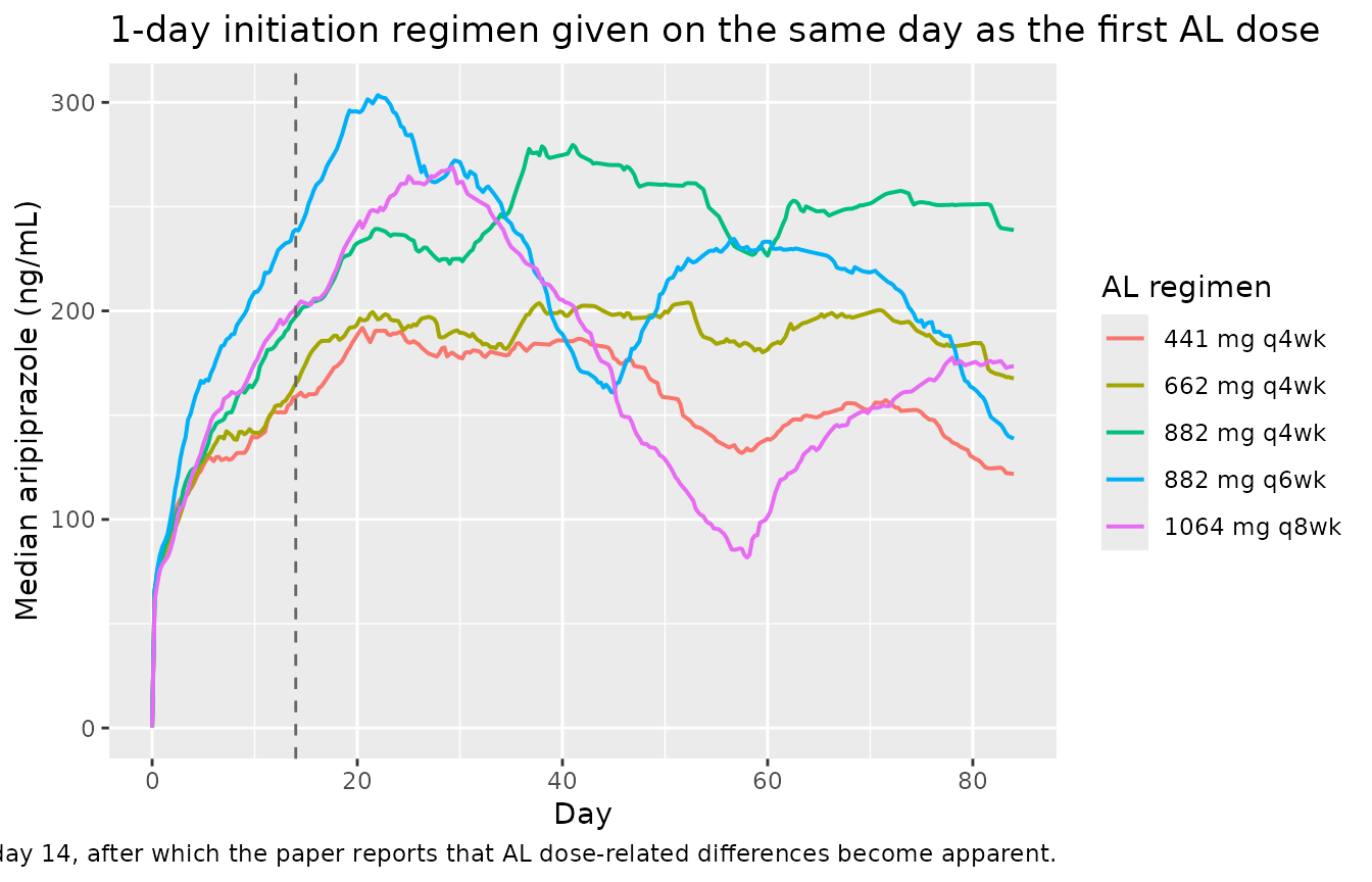
The claim is quantified here as the across-regimen spread in the
median profile, (max - min) / median, measured against the
spread of the AL doses themselves. The five regimens span 300 to 724 mg
aripiprazole equivalent, a dose spread of 71% on the same measure; if AL
were driving exposure, the concentration spread would approach that
number.
spread_pct <- function(x) 100 * (max(x) - min(x)) / stats::median(x)
dose_spread <- spread_pct(eq_dose[ss_reg$al_mg])

by_day <- init_median |>
  dplyr::group_by(time) |>
  dplyr::summarise(spread = spread_pct(Q50), .groups = "drop")

at_day <- function(d) by_day$spread[by_day$time == d * 24]

claims <- tibble::tibble(
  Measure = c(
    "Spread of the AL doses themselves",
    "Concentration spread at day 2",
    "Maximum concentration spread over days 0-14",
    "Concentration spread at day 84"
  ),
  Value = sprintf("%.0f%%", c(dose_spread, at_day(2),
                              max(by_day$spread[by_day$time <= 14 * 24]),
                              at_day(84)))
)
knitr::kable(
  claims,
  caption = "Across-regimen spread in the median profile. Early on it is far below the dose spread, because every arm is riding the same AL(NCD) injection and oral dose while the AL input has not started (ALAG alone is 4.4 days); by week 12 it exceeds the dose spread, as the regimens also differ in dosing interval."
)| Measure | Value |
|---|---|
| Spread of the AL doses themselves | 71% |
| Concentration spread at day 2 | 17% |
| Maximum concentration spread over days 0-14 | 43% |
| Concentration spread at day 84 | 70% |
# Structural rather than cohort-driven, and each bound has wide headroom against
# the realised value (12% / 47% / 86%). A mis-encoded ALNCD input would let the
# AL dose dominate from day 1 and blow the first two bounds; a mis-encoded AL
# input would flatten the late separation and blow the third.
stopifnot(
  at_day(2) < 25,
  max(by_day$spread[by_day$time <= 14 * 24]) < 60,
  at_day(84) > 60,
  at_day(84) / at_day(2) > 3
)
Assumptions and deviations
-
FRACis encoded as a logit; the transform is inferred, not published. This is the only structural inference in the model file. Supplementary Table S3 reportsFRAC = 2.02and calls it the “Weibull fraction of dose”, but the paper never writes the double-Weibull equation and 2.02 cannot be a fraction. Four candidate transforms were tested against the independently published gluteal arm of study ALK9072-B103 (ALNCD alone, 662 mg, n = 24, median tmax 25.5 days), holding every other parameter at its published value:Reading Slow-pathway share Typical-value tmax expit(FRAC)0.883 25.2 days FRAC / (1 + FRAC)0.669 5.2 days 1 / FRAC0.495 5.1 days 1 / (1 + FRAC)0.331 5.0 days Only the logit reading is compatible with the observed peak, and it also reproduces the observed Cmax; the alternatives are wrong by a factor of five on tmax. A logit is in any case the conventional NONMEM parameterisation for a parameter bounded in (0, 1), and
FRACcarries no*in Table S3, meaning it was not estimated on the log scale. Note thatMDT1andMDT2are read as Weibull scale parameters rather than as distribution means; reading them as means (dividing bygamma(1 + 1/GAM)) shifts the typical-value tmax to 27.9 days, which the B103 data disfavours but does not exclude. The
OMEGAblock off-diagonals are unpublished. Supplementary Table S3 states plainly that “only diagonal elements of the full Omega block are presented”, while Online Resource 2 says 13 of the 14 IIV terms sat in a full block. The model therefore encodes independent etas. Typical-value predictions are unaffected, but simulated between-subject behaviour is more dispersed than the paper’s, most visibly in the ALNCD tmax discussed above, where the five release-shape parameters are free to move independently of one another. Do not read the cohort statistics here as reproductions of the paper’s VPCs.Inter-occasion variability on
D ALis not encoded. Online Resource 2 states that the final model “included IOV on AL Dur, allowing variability between AL IM dosing occasions in Study 4 to be quantified”, but Supplementary Table S3 has no inter-occasion block and never reports the variance. No value is invented for it. The predecessor model,modellib("Hard_2017_aripiprazole_lauroxil"), does publish an IOV variance on itsD1(0.125) and encodes it, if an occasion term is needed.The seven AL IM depots are encoded as one lagged zero-order input to
central. Online Resource 2 says the model “was expanded by adding an additional 6 IM dosing depot for AL”, with “AL Dur, ALAG, and FIM AL … consistent across depots”. Depots that share all three parameters and carry no rate constant superpose exactly onto a single lagged modelled-duration input, which the overlapping-input arithmetic of the steady-state section above exercises directly. The encoded form also has no seven-injection ceiling. The trade-off is thatf(central)carriesFIM AL, so a hypothetical intravenous dose written tocentralwould also be scaled by 0.571; the data set contains no intravenous route.The Weibull hazards are capped at
50 / wa. A Weibull hazard with shape greater than 1 grows without bound, so long after a depot is numerically empty lsoda still sees an arbitrarily fast rate acting on an amount of order1e-300and reports “h too small for machine precision”. The cap engages only after more than 99.9999999999% of the dose has been released and leaves every number in this vignette unchanged; it is a solver guard, not a model choice.-
The oral mixture model is not part of the model file. For its simulations the paper overlaid a mixture model on the final PopPK model: a subpopulation of 37.4% of patients (95% CI 22.3-55.4%) with 44.6% lower oral bioavailability (95% CI 40.9-48.3%), fitted to the 21-day oral initiation arms of study 2 only and applied afterwards to the final model. Supplementary Table S3, which defines the final PopPK model, does not contain it, and the subpopulation is latent rather than identified by any observable covariate, so encoding it as a covariate column would misrepresent it. To apply it, scale
f(depot)by 0.554 in a randomly chosen 37.4% of simulated subjects:low_fpo <- stats::runif(n_subjects) < 0.374 # then simulate the low-Fpo subjects with oral amt * 0.554It matters only for multiple-dose oral aripiprazole; the single 30 mg oral dose of the 1-day initiation regimen is not where the paper saw the subpopulation.
ARI(0)is encoded as an initial condition oncentral. The(0)notation is NONMEM’s initial-amount syntax and the value is reported in ng/mL, so the encoding iscentral(0) <- c0 * vc / 1000. Its IIV variance of 4.34 is very large (the table’s own CV is 870%), reflecting how few patients had quantifiable pre-dose aripiprazole; users simulating the first days after a first injection should expect a small number of virtual subjects to start with a substantial residual concentration.FPO’s IIV was fixed to zero (Online Resource 2), so no eta is attached tolfdepot.No covariate effects survive except weight on
Vc/F. The full model carried eight effects (Supplementary Table S2): weight onVc/F,CL/F,D ALandALAG AL, age onCL/F, ALNCD injection site onFRAC, and AL injection site onD ALandALAG AL. Backward elimination at p = 0.001 left only weight onVc/F. In particular clearance does not scale with weight in this model, and injection site has no effect, even though the separately published study B103 does show a deltoid/gluteal difference in tmax. Those estimates belong to the full model, whose other parameters are unpublished, so they cannot be grafted onto the final model.Table 2’s late-dose and recovery columns are not reproduced. The paper does not state the window over which
Cmaxwas taken in those scenarios, nor the ALNCD dose used for re-establishment, nor the simulation horizon treated as steady state. Reproducing them would require guessing all three. The “No late dose” column, which is fully specified, is reproduced above.The virtual cohorts draw weight as
N(89.1, 17.9)kg (Table 1, all studies) except the study B103 replication, which uses that study’s ownN(86.6, 15.6)kg; both are clipped to a plausible adult range, since the paper reports no weight range. All simulated subjects are CYP2D6 non-poor metabolizers, because the data set contained none and the model has no term for them.