Model and source
- Citation: Matcha S, Dilli Batcha JS, Raju AP, Chaudhari BB, Moorkoth S, Mallayasamy S, Lewis LE. Precision dosing of amikacin in term neonates using pharmacometric approach. Pediatr Res. 2025;98:936-941. doi:10.1038/s41390-025-04044-7. The age-typical serum-creatinine reference equation (Matcha 2025 Eq. 8) is taken from Wang H, Sherwin C, Gobburu JVS, Ivaturi V. Population pharmacokinetic modeling of gentamicin in pediatrics. J Clin Pharmacol. 2019;59:1584-1596.
- Description: Two-compartment IV population PK model for amikacin in term neonates (Matcha 2025); clearance carries an uncentred exponential body-weight effect (Exp^(WT * 0.308)) and a power renal-function ratio (SCrmean / SCr)^0.397, where SCrmean is the age-typical population serum creatinine predicted from postnatal age by the Wang 2019 paediatric reference equation, so postnatal age enters clearance as renal maturation; central volume, peripheral volume, and intercompartmental clearance carry no covariates. Supports the paper’s WT / SCr / PNA dosing nomogram targeting peak 24-35 mg/L and trough 2-5 mg/L.
- Article: https://doi.org/10.1038/s41390-025-04044-7
- Supplement (Tables S1-S2, Figure S1): https://doi.org/10.1038/s41390-025-04044-7
Matcha 2025 developed a two-compartment intravenous population PK model for amikacin in term neonates and used it to build a dosing nomogram indexed by body weight, serum creatinine, and postnatal age. The paper’s stated design targets are a peak concentration of about 30 mg/L (acceptable window 24-35 mg/L) and a trough of about 3 mg/L (acceptable window 2-5 mg/L).
Population
The model was fitted to 100 amikacin concentrations from 78 term neonates in a single-centre prospective observational study in India (101 concentrations from 80 neonates before data cleaning; one outlying observation of 154 mg/L and one subject with no usable concentrations were removed – supplementary Table S1). Gestational age was 37-42 weeks (median 39), current body weight 1.74-4.84 kg (median 2.85), and serum creatinine 0.16-1.49 mg/dL (median 0.55). Postnatal age at sample collection ranged from 0.62 to 27.32 days (median 5.02). Doses were 25-110 mg (median 40 mg), i.e. 8.23-51.89 mg/kg (median 12.52 mg/kg), and sampling was opportunistic at 0.5-24 h after the most recent dose (Matcha 2025 Table 1 and Figure 1). Sex distribution was not reported. The model was fitted with Pumas in Julia 1.6 and evaluated by VPC (n = 500) and bootstrap (n = 1000, 100% success).
The same information is available programmatically from the model’s
population metadata:
pop <- rxode2::rxode(readModelDb("Matcha_2025_amikacin"))$population
#> ℹ parameter labels from comments will be replaced by 'label()'
str(pop, max.level = 1)
#> List of 18
#>  $ species       : chr "human"
#>  $ n_subjects    : num 78
#>  $ n_studies     : num 1
#>  $ n_observations: num 100
#>  $ age_range     : chr "PNA at start of amikacin 0.04-21.29 days; PNA at sample collection 0.62-27.32 days"
#>  $ age_median    : chr "PNA 1.70 days at start of amikacin; 5.02 days at sample collection"
#>  $ ga_range      : chr "Gestational age 37-42 weeks (term only); postmenstrual age at start of amikacin 37.11-42.22 weeks"
#>  $ ga_median     : chr "Gestational age 39 weeks; postmenstrual age 39.20 weeks"
#>  $ weight_range  : chr "Current body weight 1.74-4.84 kg; birth weight 1.75-4.50 kg"
#>  $ weight_median : chr "Current body weight 2.85 kg; birth weight 2.95 kg"
#>  $ sex_female_pct: num NA
#>  $ race_ethnicity: chr "Not reported; single-centre Indian cohort"
#>  $ disease_state : chr "Term neonates prescribed amikacin for suspected or confirmed sepsis; clinically unstable neonates were excluded."
#>  $ dose_range    : chr "25-110 mg IV (median 40 mg), equivalent to 8.23-51.89 mg/kg (median 12.52 mg/kg)"
#>  $ regions       : chr "India (single-centre prospective observational study; Kasturba Medical College, Manipal)"
#>  $ renal_function: chr "Serum creatinine 0.16-1.49 mg/dL (median 0.55); Schwartz-estimated creatinine clearance 12.68-145.0 mL/min (med"| __truncated__
#>  $ notes         : chr "Demographics from Matcha 2025 Table 1. 101 concentrations were collected from 80 neonates; after removing one o"| __truncated__
#>  $ sex_note      : chr "Sex distribution not reported in Matcha 2025."
Source trace
Every ini() entry in
inst/modeldb/specificDrugs/Matcha_2025_amikacin.R carries
an in-file comment naming its source location. They are collected here
for review.
| Equation / parameter | Value | Source location |
|---|---|---|
lcl (TVCL) |
0.064 L/h | Table 2; Eq. 4 |
lvc (TVVC) |
1.281 L | Table 2; Eq. 5 |
lq (TVQ) |
0.055 L/h | Table 2; Eq. 7 |
lvp (TVVP) |
0.618 L | Table 2; Eq. 6 |
e_wt_cl (Wt_cl) |
0.308 (1/kg) | Table 2; Eq. 4 |
e_creat_cl (SCr_cl) |
0.397 (unitless) | Table 2; Eq. 4 |
etalcl |
0.106966 (BSV 33.6 %CV) | Table 2 BSV_cl |
etalvc |
0.156081 (BSV 41.1 %CV) | Table 2 BSV_vc |
propSd |
0.309 (30.9 %CV) | Table 2 proportional residual error |
CL_i = 0.064 * Exp^(WT * 0.308) * (SCrmean / SCr)^0.397 * Exp^(etacl) |
n/a | Eq. 4 |
VC_i = 1.281 * Exp^(etavc) |
n/a | Eq. 5 |
VP_i = 0.618 |
n/a | Eq. 6 |
Q_i = 0.055 |
n/a | Eq. 7 |
SCrmean = -0.02324 - 0.14545 * log(PNA) + 0.26964 * PNA^0.5 |
n/a | Eq. 8 (adopted from Wang 2019); repeated verbatim in supplementary Table S1 |
| Two-compartment IV disposition | n/a | Results, “A two-compartment structural PK model best explained the study data” |
| Proportional residual error | n/a | Results, “A proportional residual error model was chosen” |
| Target windows: peak 24-35 mg/L, trough 2-5 mg/L | n/a | Methods “Dosing nomogram”; Discussion |
| Target attainment: peak 50 / 30 / 20 %, trough 50 / 20 / 30 % (in / above / below) | n/a | Results, final paragraph of “Dosing nomogram” results |
| Dosing nomogram (100 covariate cells) | n/a | Table 3 |
Two points in the source trace needed care, because naive text
extraction of the article PDF drops every display equation (none of Eqs.
4-8 survives it). Both were read directly off the publisher’s own
typesetting, by rasterising page 3 of the article PDF at 600 dpi
(pdftoppm -r 600 -f 3 -l 3) and cropping to the equation
bounding boxes located with pdftotext -bbox. At that
resolution the superscript structure and the leading signs are
unambiguous. Each was then corroborated against a second, independent
source:
-
Eq. 4 uses an exponential, not a power, body-weight
model. The typeset equation reads
CL_i = 0.064 * Exp^(WT*0.308) * (SCrmean / SCr)^0.397 * EXP^(etacl), withWT*0.308set as a superscript onExpand0.397as a superscript on the bracketed creatinine ratio. (The PDF’s flat text layer mangles this intoCLi = 0:064 ExpWT0:308 (SCrmean / SCr) 0:397 EXPetacl, which is what makes the rasterised reading necessary: superscripts are flattened into the baseline run and decimal points come out as colons.) The exponential form matches the Methods statement that “power and exponential functions were used to describe the covariate effects for continuous covariates”, and is confirmed independently by the Table 3 nomogram arithmetic below. The consequence is that the WT effect is uncentred:lcl= 0.064 L/h is the clearance extrapolated to WT = 0 kg, not the typical clearance of a neonate. -
Eq. 8 has two leading minus signs. The typeset
equation reads
SCrmean = -0.02324 - 0.14545 x log(PNA) + 0.26964 x PNA^0.5. The version of this image redistributed by EuropePMC (Equ8.gif, 200x9 px) is too coarse to resolve the leading sign, but the 600 dpi page render is not. Supplementary Table S1 settles it a second time, independently of the article body: the row “SCr completely missing / Filled with SCr predictions (Wang et al., 2019)” prints the equation in code form as-0.02324 - (0.14545 * log(PNA)) + 0.26964 * (PNA0.5).
log() is the natural logarithm: the model was fitted in
Julia/Pumas, where log is the natural log, and the
supplement writes Eq. 8 in that code form.
Renal maturation enters clearance through the reference creatinine
Postnatal age is not a direct covariate on any PK parameter. It
enters clearance through SCrmean, the age-typical
population serum creatinine (Eq. 8), which is the numerator of the
renal-function ratio on CL. The paper describes this as incorporating
renal maturation, “which is directly proportional to PNA and gestational
age”, so SCrmean – and therefore typical clearance – must
increase across the neonatal window.
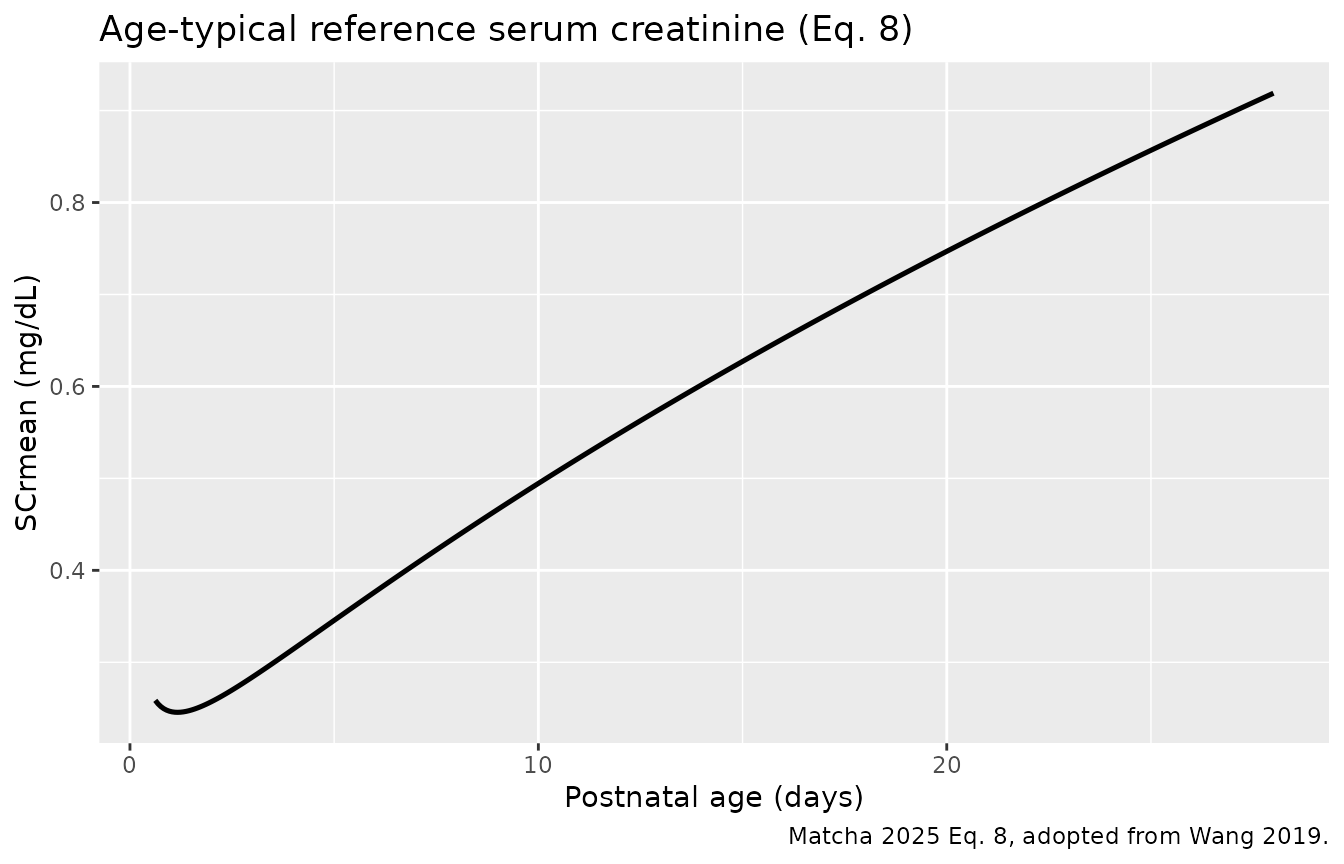
Eq. 8 is not monotone everywhere, however. Its derivative
-0.14545 / PNA + 0.13482 / sqrt(PNA) vanishes at
PNA = (0.14545 / 0.13482)^2 = 1.164 days, so the curve
falls very slightly over the first day of life and rises strictly
thereafter. The dip is 5% of the value at the cohort’s earliest sampling
time and is confined below 1.2 days; across the whole of the published
nomogram (PNA bands starting at 1 day) and essentially the whole cohort,
SCrmean increases with postnatal age as the paper
describes.
scr_mean_fun <- function(pna_days) {
  -0.02324 - 0.14545 * log(pna_days) + 0.26964 * pna_days^0.5
}

pna_days <- seq(0.62, 28, length.out = 400)

ggplot(data.frame(pna_days, scr_mean = scr_mean_fun(pna_days)),
       aes(pna_days, scr_mean)) +
  geom_line(linewidth = 0.9) +
  labs(
    x = "Postnatal age (days)",
    y = "SCrmean (mg/dL)",
    title = "Age-typical reference serum creatinine (Eq. 8)",
    caption = "Matcha 2025 Eq. 8, adopted from Wang 2019."
  )
# The analytic turning point must agree with the numerical argmin.
turning_point <- (0.14545 / 0.13482)^2
fine <- seq(0.5, 3, length.out = 100001)
stopifnot(abs(fine[which.min(scr_mean_fun(fine))] - turning_point) < 1e-3)

# Strictly increasing above the turning point -- this is the property the
# paper's renal-maturation story and the Table 3 interval trend both require.
stopifnot(all(diff(scr_mean_fun(seq(1.17, 28, length.out = 5000))) > 0))

# ... and the pre-turning-point dip is negligible over the nomogram's range.
stopifnot(
  scr_mean_fun(1) - min(scr_mean_fun(seq(1, 28, length.out = 5000))) < 0.001
)

c(turning_point_days = turning_point,
  day_0.62 = scr_mean_fun(0.62),
  day_1    = scr_mean_fun(1),
  day_5.02 = scr_mean_fun(5.02),
  day_28   = scr_mean_fun(28),
  fold_1_to_28 = scr_mean_fun(28) / scr_mean_fun(1))
#> turning_point_days           day_0.62              day_1           day_5.02
#>          1.1639084          0.2586051          0.2464000          0.3462246
#>             day_28       fold_1_to_28
#>          0.9188916          3.7292679
Between day 1 and day 28 the reference creatinine rises 3.73-fold,
which by Eq. 4 raises typical clearance by 3.73^0.397 =
1.69-fold across the neonatal period at fixed weight and measured
creatinine.
This also cross-checks against Table 3: holding weight and creatinine fixed, every column of the nomogram shortens its dosing interval as the postnatal-age band increases (e.g. at WT 2.00-2.49 kg and SCr 0.50-0.74 mg/dL the interval goes 36 h, 30 h, 30 h, 24 h across the four weeks), which requires clearance to rise with postnatal age.
The weight model is exponential, not allometric
The one structural reading that the PDF’s flat text layer cannot
settle is whether Eq. 4’s weight term is Exp^(WT * 0.308)
(exponential, uncentred) or (WT / ref)^0.308 (allometric
power). The publisher’s typesetting says exponential, and Table 3 proves
it independently – which matters here, because the paper’s own
Discussion reads more naturally under the power form (see Assumptions
below).
Within one nomogram row the target window is held fixed, so the total dose rate prescribed for a cell must be proportional to that cell’s clearance. Reading the whole weight axis of a row therefore measures the shape of the weight effect directly, with no free parameters – a stronger test than comparing only the two end bands, because a wrong functional form has to miss the interior bands too.
wt_mid <- c(2.245, 2.745, 3.245, 3.745, 4.250)  # midpoints of the five WT bands

# Two independent rows of Table 3, both at PNA 1-7 days.
rows <- list(
  "SCr 0.15-0.29" = list(mg_per_kg = c(17, 15, 12, 11, 9), tau = c(24, 21, 18, 15, 12)),
  "SCr 0.50-0.74" = list(mg_per_kg = c(16, 13, 12, 10, 9), tau = c(36, 30, 30, 24, 21))
)

# Dose rate (mg/h) for each cell, expressed relative to the lightest band.
relative_rate <- function(c_row) {
  rate <- c_row$mg_per_kg * wt_mid / c_row$tau
  rate / rate[1]
}

wt_check <- tibble::tibble(
  row      = rep(names(rows), each = length(wt_mid)),
  wt       = rep(wt_mid, length(rows)),
  observed = unlist(lapply(rows, relative_rate), use.names = FALSE)
) |>
  dplyr::mutate(
    exponential = exp(0.308 * (wt - wt_mid[1])),
    power       = (wt / wt_mid[1])^0.308
  )

wt_check
#> # A tibble: 10 × 5
#>    row              wt observed exponential power
#>    <chr>         <dbl>    <dbl>       <dbl> <dbl>
#>  1 SCr 0.15-0.29  2.24     1           1     1
#>  2 SCr 0.15-0.29  2.74     1.23        1.17  1.06
#>  3 SCr 0.15-0.29  3.24     1.36        1.36  1.12
#>  4 SCr 0.15-0.29  3.74     1.73        1.59  1.17
#>  5 SCr 0.15-0.29  4.25     2.00        1.85  1.22
#>  6 SCr 0.50-0.74  2.24     1           1     1
#>  7 SCr 0.50-0.74  2.74     1.19        1.17  1.06
#>  8 SCr 0.50-0.74  3.24     1.30        1.36  1.12
#>  9 SCr 0.50-0.74  3.74     1.56        1.59  1.17
#> 10 SCr 0.50-0.74  4.25     1.83        1.85  1.22

# Mean absolute relative error of each candidate form across all 10 cells.
err <- wt_check |>
  dplyr::summarise(
    exponential = mean(abs(exponential - observed) / observed),
    power       = mean(abs(power - observed) / observed)
  )
err
#> # A tibble: 1 × 2
#>   exponential power
#>         <dbl> <dbl>
#> 1      0.0308 0.186

# The exponential form must track the nomogram closely AND beat the allometric
# form by a wide margin. Both bounds have ample headroom (measured: ~3% vs ~19%),
# so neither is filed down to the observed value.
stopifnot(err$exponential < 0.10, err$exponential < err$power / 3)
Across all ten cells the exponential form tracks the published nomogram to about 3% on average, while the allometric power form is off by about 19% and understates the size of the effect roughly four-fold: at the heaviest band it predicts a 1.22-fold clearance increase where the nomogram demands 1.8-2.0. The exponential reading is adopted.
A second, independent consequence of the exponential-and-uncentred
weight model is that VC carries no covariate at all, so the
peak concentration dose / VC depends only on the absolute
milligram dose. Table 3 shows exactly this: the 17 mg/kg q24h cell at
2.245 kg and the 9 mg/kg q12h cell at 4.250 kg both prescribe about 38
mg, which is 38 / 1.281 = 30 mg/L – the paper’s stated peak
target.
dose_lo <- 17 * wt_mid[1]   # 17 mg/kg at the 2.00-2.49 kg band midpoint
dose_hi <-  9 * wt_mid[5]   #  9 mg/kg at the 4.00-4.50 kg band midpoint
vc      <- 1.281

c(dose_lo_mg = dose_lo, dose_hi_mg = dose_hi,
  peak_lo = dose_lo / vc, peak_hi = dose_hi / vc)
#> dose_lo_mg dose_hi_mg    peak_lo    peak_hi
#>   38.16500   38.25000   29.79313   29.85948

# Both cells must land inside the paper's 24-35 mg/L peak window.
stopifnot(dplyr::between(dose_lo / vc, 24, 35),
          dplyr::between(dose_hi / vc, 24, 35))
Virtual cohort
Original observed data are not publicly available, so the figures below use virtual neonates whose covariate distributions approximate Table 1.
# Each stochastic block below seeds itself immediately before it draws, rather
# than relying on one global seed here. A single top-of-file seed would make
# every draw depend on the cumulative RNG consumption of every chunk above it,
# so merely inserting or reordering a chunk would silently shift every result
# and assertion downstream.

DAYS_PER_MONTH <- 30.4375  # canonical PNA column is in months; the paper uses days

# One IV infusion series plus observation records for a set of subjects.
# `subj` must carry id, WT, CREAT (mg/dL), pna_days, dose_mg, tau, n_dose.
# `obs_offsets` are observation times measured from the START of the dose whose
# index is given by `obs_dose_index` (1 = first dose, n_dose = last dose).
build_events <- function(subj, obs_times) {
  doses <-
    subj |>
    dplyr::select(id, WT, CREAT, pna_days, dose_mg, tau, n_dose, label) |>
    dplyr::mutate(dose_no = lapply(n_dose, seq_len)) |>
    tidyr::unnest(dose_no) |>
    dplyr::mutate(
      time = (dose_no - 1) * tau,
      amt  = dose_mg,
      evid = 1L,
      cmt  = "central",
      rate = dose_mg / 0.5  # 30-min IV infusion
    ) |>
    dplyr::select(-dose_no)

  obs <-
    obs_times |>
    dplyr::mutate(
      amt  = NA_real_,
      evid = 0L,
      cmt  = "central",
      rate = 0
    )

  dplyr::bind_rows(doses, obs) |>
    dplyr::mutate(PNA = pna_days / DAYS_PER_MONTH) |>
    dplyr::arrange(id, time, dplyr::desc(evid)) |>
    dplyr::select(id, time, amt, evid, cmt, rate, WT, CREAT, PNA, pna_days,
                  dose_mg, tau, n_dose, label)
}

# Number of doses needed to be safely at steady state for a given interval.
n_dose_for_ss <- function(tau) pmax(3L, pmin(12L, as.integer(ceiling(120 / tau)) + 1L))
Population cohort (Figures 1 and 3)
set.seed(20250418)

n_pop <- 200

subj_pop <- tibble::tibble(
  id       = seq_len(n_pop),
  WT       = runif(n_pop, 1.74, 4.84),
  CREAT    = runif(n_pop, 0.16, 1.49),
  pna_days = runif(n_pop, 0.62, 27.32),
  tau      = 24,
  n_dose   = 1L,
  label    = "Population (median 12.52 mg/kg)"
) |>
  dplyr::mutate(dose_mg = 12.52 * WT)

obs_pop <-
  subj_pop |>
  dplyr::select(id, WT, CREAT, pna_days, dose_mg, tau, n_dose, label) |>
  tidyr::crossing(time = c(seq(0, 6, by = 0.25), seq(6.5, 60, by = 0.5)))

events_pop <- build_events(subj_pop, obs_pop)
stopifnot(anyDuplicated(events_pop[, c("id", "time", "evid")]) == 0L)
Regimen cohort (PKNCA)
Three representative nomogram cells, each at the dose and interval Table 3 prescribes for that cell.
regimens <- tibble::tribble(
  ~label,                                   ~WT,   ~CREAT, ~pna_days, ~mg_per_kg, ~tau,
  "2.25 kg, SCr 0.62, PNA 4 d: 16 mg/kg q36h",  2.245, 0.620, 4,   16, 36,
  "3.25 kg, SCr 0.62, PNA 11 d: 12 mg/kg q24h", 3.245, 0.620, 11,  12, 24,
  "4.25 kg, SCr 0.22, PNA 25 d: 11 mg/kg q9h",  4.250, 0.220, 25,  11,  9
)

n_per_reg <- 100

subj_reg <-
  regimens |>
  dplyr::mutate(rep = list(seq_len(n_per_reg))) |>
  tidyr::unnest(rep) |>
  dplyr::mutate(
    id      = dplyr::row_number(),
    dose_mg = mg_per_kg * WT,
    n_dose  = 1L
  ) |>
  dplyr::select(id, WT, CREAT, pna_days, dose_mg, tau, n_dose, label)

obs_reg <-
  subj_reg |>
  tidyr::crossing(time = c(seq(0, 8, by = 0.25), seq(8.5, 48, by = 0.5),
                           seq(50, 240, by = 4)))

events_reg <- build_events(subj_reg, obs_reg)
stopifnot(anyDuplicated(events_reg[, c("id", "time", "evid")]) == 0L)
Nomogram cohort (target attainment)
All 100 cells of Table 3, with 50 virtual neonates per cell whose weight, creatinine, and postnatal age are drawn uniformly inside the cell’s band. Peak is taken at the end of the 30-min infusion and trough at the end of the dosing interval, at both the first dose and steady state.
set.seed(20250419)

nomogram <- tibble::tribble(
  ~pna_band, ~scr_band, ~wt_band, ~mg_per_kg, ~tau,
  # PNA 1-7 days
  1, 1, 1, 17, 24, 1, 1, 2, 15, 21, 1, 1, 3, 12, 18, 1, 1, 4, 11, 15, 1, 1, 5,  9, 12,
  1, 2, 1, 17, 30, 1, 2, 2, 13, 24, 1, 2, 3, 12, 24, 1, 2, 4, 10, 18, 1, 2, 5, 10, 18,
  1, 3, 1, 16, 36, 1, 3, 2, 13, 30, 1, 3, 3, 12, 30, 1, 3, 4, 10, 24, 1, 3, 5,  9, 21,
  1, 4, 1, 16, 42, 1, 4, 2, 13, 36, 1, 4, 3, 12, 30, 1, 4, 4, 10, 24, 1, 4, 5,  9, 24,
  1, 5, 1, 16, 48, 1, 5, 2, 13, 42, 1, 5, 3, 12, 36, 1, 5, 4, 10, 30, 1, 5, 5,  9, 24,
  # PNA 8-14 days
  2, 1, 1, 18, 21, 2, 1, 2, 15, 21, 2, 1, 3, 13, 15, 2, 1, 4, 11, 12, 2, 1, 5, 11, 12,
  2, 2, 1, 17, 24, 2, 2, 2, 13, 18, 2, 2, 3, 12, 18, 2, 2, 4, 11, 15, 2, 2, 5, 11, 15,
  2, 3, 1, 16, 30, 2, 3, 2, 13, 24, 2, 3, 3, 12, 24, 2, 3, 4, 10, 18, 2, 3, 5,  9, 15,
  2, 4, 1, 17, 36, 2, 4, 2, 14, 30, 2, 4, 3, 12, 24, 2, 4, 4, 10, 21, 2, 4, 5,  9, 18,
  2, 5, 1, 17, 42, 2, 5, 2, 14, 36, 2, 5, 3, 12, 30, 2, 5, 4, 10, 24, 2, 5, 5,  9, 21,
  # PNA 15-21 days
  3, 1, 1, 18, 18, 3, 1, 2, 15, 15, 3, 1, 3, 13, 12, 3, 1, 4, 13, 12, 3, 1, 5, 11,  9,
  3, 2, 1, 18, 18, 3, 2, 2, 14, 18, 3, 2, 3, 13, 18, 3, 2, 4, 12, 15, 3, 2, 5, 10, 12,
  3, 3, 1, 17, 30, 3, 3, 2, 14, 24, 3, 3, 3, 12, 21, 3, 3, 4, 11, 18, 3, 3, 5, 10, 15,
  3, 4, 1, 16, 30, 3, 4, 2, 13, 24, 3, 4, 3, 12, 21, 3, 4, 4, 10, 18, 3, 4, 5,  9, 15,
  3, 5, 1, 16, 36, 3, 5, 2, 13, 30, 3, 5, 3, 12, 24, 3, 5, 4, 10, 21, 3, 5, 5,  9, 18,
  # PNA 22-28 days
  4, 1, 1, 17, 15, 4, 1, 2, 16, 15, 4, 1, 3, 14, 12, 4, 1, 4, 14, 12, 4, 1, 5, 11,  9,
  4, 2, 1, 19, 18, 4, 2, 2, 15, 18, 4, 2, 3, 13, 15, 4, 2, 4, 11, 12, 4, 2, 5, 11, 12,
  4, 3, 1, 17, 24, 4, 3, 2, 14, 21, 4, 3, 3, 12, 18, 4, 3, 4, 11, 15, 4, 3, 5, 10, 12,
  4, 4, 1, 16, 24, 4, 4, 2, 14, 24, 4, 4, 3, 13, 21, 4, 4, 4, 11, 18, 4, 4, 5, 10, 15,
  4, 5, 1, 16, 30, 4, 5, 2, 14, 30, 4, 5, 3, 12, 24, 4, 5, 4, 11, 21, 4, 5, 5, 10, 18
)
stopifnot(nrow(nomogram) == 100L)

wt_bounds  <- tibble::tibble(wt_band = 1:5,
                             wt_lo = c(2.00, 2.50, 3.00, 3.50, 4.00),
                             wt_hi = c(2.49, 2.99, 3.49, 3.99, 4.50))
scr_bounds <- tibble::tibble(scr_band = 1:5,
                             scr_lo = c(0.15, 0.30, 0.50, 0.75, 1.00),
                             scr_hi = c(0.29, 0.49, 0.74, 0.99, 1.50))
pna_bounds <- tibble::tibble(pna_band = 1:4,
                             pna_lo = c(1, 8, 15, 22),
                             pna_hi = c(7, 14, 21, 28))

n_per_cell <- 50

subj_nom <-
  nomogram |>
  dplyr::left_join(wt_bounds,  by = "wt_band") |>
  dplyr::left_join(scr_bounds, by = "scr_band") |>
  dplyr::left_join(pna_bounds, by = "pna_band") |>
  dplyr::mutate(cell = dplyr::row_number(), rep = list(seq_len(n_per_cell))) |>
  tidyr::unnest(rep) |>
  dplyr::mutate(
    id       = dplyr::row_number(),
    WT       = runif(dplyr::n(), wt_lo,  wt_hi),
    CREAT    = runif(dplyr::n(), scr_lo, scr_hi),
    pna_days = runif(dplyr::n(), pna_lo, pna_hi),
    dose_mg  = mg_per_kg * WT,
    n_dose   = n_dose_for_ss(tau),
    label    = paste0("cell ", cell)
  ) |>
  dplyr::select(id, cell, WT, CREAT, pna_days, dose_mg, tau, n_dose, label)

obs_nom <-
  subj_nom |>
  dplyr::select(id, WT, CREAT, pna_days, dose_mg, tau, n_dose, label) |>
  dplyr::mutate(
    peak_first   = 0.5,
    trough_first = tau,
    peak_ss      = (n_dose - 1) * tau + 0.5,
    trough_ss    = n_dose * tau
  ) |>
  tidyr::pivot_longer(c(peak_first, trough_first, peak_ss, trough_ss),
                      names_to = "metric", values_to = "time")

events_nom <- build_events(subj_nom, obs_nom) |>
  dplyr::left_join(obs_nom |> dplyr::select(id, time, metric), by = c("id", "time"))
stopifnot(anyDuplicated(events_nom[, c("id", "time", "evid")]) == 0L)
nrow(events_nom)
#> [1] 56600
Simulation
# rxSolve draws the between-subject etas, so this block is stochastic too and
# carries its own seed for rxode2's generator.
rxode2::rxSetSeed(20250420)

mod <- readModelDb("Matcha_2025_amikacin")

sim_pop <- rxode2::rxSolve(
  mod, events = events_pop,
  keep = c("WT", "CREAT", "pna_days", "dose_mg", "label")
) |> as.data.frame()
#> ℹ parameter labels from comments will be replaced by 'label()'

sim_reg <- rxode2::rxSolve(
  mod, events = events_reg,
  keep = c("WT", "CREAT", "pna_days", "dose_mg", "tau", "label")
) |> as.data.frame()

sim_nom <- rxode2::rxSolve(
  mod, events = events_nom,
  keep = c("WT", "CREAT", "pna_days", "dose_mg", "tau", "metric", "label")
) |> as.data.frame()

stopifnot(all(is.finite(sim_pop$Cc)), all(sim_pop$Cc >= 0))
dplyr::n_distinct(sim_nom$id)
#> [1] 5000
The Cc column is the individual prediction without
residual error; the sim column additionally carries the
proportional residual error and is what the VPC below plots.
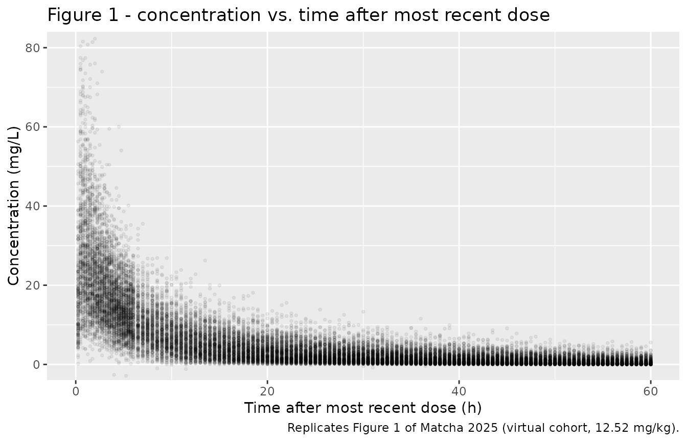
Replicate published figures
# Replicates Figure 1 of Matcha 2025: amikacin concentration vs. time after the
# most recent dose.
sim_pop |>
  dplyr::filter(!is.na(Cc), time > 0) |>
  ggplot(aes(time, sim)) +
  geom_point(alpha = 0.06, size = 0.7) +
  coord_cartesian(xlim = c(0, 60), ylim = c(0, 80)) +
  labs(
    x = "Time after most recent dose (h)",
    y = "Concentration (mg/L)",
    title = "Figure 1 - concentration vs. time after most recent dose",
    caption = "Replicates Figure 1 of Matcha 2025 (virtual cohort, 12.52 mg/kg)."
  )
# Replicates Figure 3 of Matcha 2025: VPC of the final model.
vpc <-
  sim_pop |>
  dplyr::filter(!is.na(Cc), time > 0, sim > 0) |>
  dplyr::mutate(tbin = cut(time, breaks = seq(0, 60, by = 2), labels = FALSE)) |>
  dplyr::group_by(tbin) |>
  dplyr::summarise(
    time = median(time),
    Q10  = quantile(sim, 0.10),
    Q50  = quantile(sim, 0.50),
    Q90  = quantile(sim, 0.90),
    .groups = "drop"
  )

ggplot(vpc, aes(time, Q50)) +
  geom_ribbon(aes(ymin = Q10, ymax = Q90), alpha = 0.25) +
  geom_line(linewidth = 0.9) +
  scale_y_log10(limits = c(0.1, 100)) +
  labs(
    x = "Time after last dose (h)",
    y = "Concentration (mg/L)",
    title = "Figure 3 - visual predictive check",
    caption = "Replicates Figure 3 of Matcha 2025: median and 10th-90th prediction interval."
  )
#> Warning: Removed 7 rows containing missing values or values outside the scale range
#> (`geom_ribbon()`).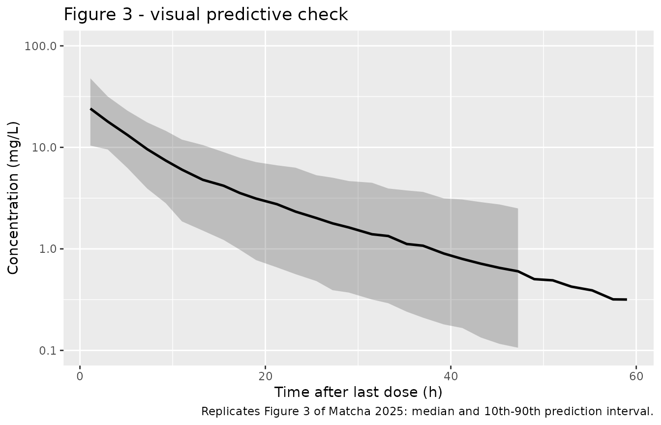
The simulated envelope covers 0.04-48 mg/L across 0-60 h after the dose, which sits inside the published VPC’s 0.1-100 mg/L axis range and matches its spread.
PKNCA validation
sim_nca <-
  sim_reg |>
  dplyr::filter(!is.na(Cc)) |>
  dplyr::select(id, time, Cc, label)

# Guarantee a time = 0 row per (id, label); for an IV dose the pre-dose
# concentration is 0.
sim_nca <- dplyr::bind_rows(
  sim_nca,
  sim_nca |> dplyr::distinct(id, label) |> dplyr::mutate(time = 0, Cc = 0)
) |>
  dplyr::distinct(id, label, time, .keep_all = TRUE) |>
  dplyr::arrange(id, label, time)

conc_obj <- PKNCA::PKNCAconc(sim_nca, Cc ~ time | label + id)

dose_df <-
  events_reg |>
  dplyr::filter(evid == 1) |>
  dplyr::select(id, time, amt, label)

dose_obj <- PKNCA::PKNCAdose(dose_df, amt ~ time | label + id)

intervals <- data.frame(
  start      = 0,
  end        = Inf,
  cmax       = TRUE,
  tmax       = TRUE,
  auclast    = TRUE,
  aucinf.obs = TRUE,
  half.life  = TRUE,
  cl.obs     = TRUE
)

# progress = FALSE suppresses PKNCA's progress bar, whose timing-dependent
# output is otherwise the only thing that differs between two renders.
nca_res <- PKNCA::pk.nca(
  PKNCA::PKNCAdata(conc_obj, dose_obj, intervals = intervals,
                   options = list(progress = FALSE))
)

nca_res$result |>
  dplyr::filter(PPTESTCD %in% c("cmax", "tmax", "auclast", "aucinf.obs",
                                "half.life", "cl.obs")) |>
  dplyr::group_by(label, PPTESTCD) |>
  dplyr::summarise(median = median(PPORRES, na.rm = TRUE), .groups = "drop") |>
  tidyr::pivot_wider(names_from = PPTESTCD, values_from = median) |>
  dplyr::rename(
    "Regimen"          = label,
    "Cmax (mg/L)"      = cmax,
    "Tmax (h)"         = tmax,
    "AUClast (mg*h/L)" = auclast,
    "AUC0-inf (mg*h/L)" = aucinf.obs,
    "t1/2 (h)"         = half.life,
    "CL (L/h)"         = cl.obs
  ) |>
knitr::kable(digits = 3, caption = "Median single-dose NCA by regimen (virtual cohort).")| Regimen | AUC0-inf (mg*h/L) | AUClast (mg*h/L) | CL (L/h) | Cmax (mg/L) | t1/2 (h) | Tmax (h) |
|---|---|---|---|---|---|---|
| 2.25 kg, SCr 0.62, PNA 4 d: 16 mg/kg q36h | 361.021 | 361.015 | 0.099 | 28.634 | 17.336 | 0.5 |
| 3.25 kg, SCr 0.62, PNA 11 d: 12 mg/kg q24h | 235.491 | 235.487 | 0.165 | 29.612 | 12.168 | 0.5 |
| 4.25 kg, SCr 0.22, PNA 25 d: 11 mg/kg q9h | 121.165 | 121.165 | 0.386 | 34.054 | 9.270 | 0.5 |
Structural identity: AUC0-inf equals dose / CL
For a linear model given intravenously, AUC0-inf must
equal dose / CL exactly for every subject. Checking this
per subject on a typical-value (no between-subject variability)
simulation is a much stricter test than comparing medians, because it
has no sampling noise to hide behind.
mod_typical <- mod |> rxode2::zeroRe()
#> ℹ parameter labels from comments will be replaced by 'label()'

sim_typ <- rxode2::rxSolve(
  mod_typical, events = events_reg, omega = NA,
  keep = c("WT", "CREAT", "pna_days", "dose_mg", "label")
) |> as.data.frame()
#> Warning: multi-subject simulation without without 'omega'

typ_nca <-
  sim_typ |>
  dplyr::filter(!is.na(Cc)) |>
  dplyr::select(id, time, Cc, label)

typ_nca <- dplyr::bind_rows(
  typ_nca,
  typ_nca |> dplyr::distinct(id, label) |> dplyr::mutate(time = 0, Cc = 0)
) |>
  dplyr::distinct(id, label, time, .keep_all = TRUE) |>
  dplyr::arrange(id, label, time)

typ_res <- PKNCA::pk.nca(PKNCA::PKNCAdata(
  PKNCA::PKNCAconc(typ_nca, Cc ~ time | label + id),
  PKNCA::PKNCAdose(dose_df, amt ~ time | label + id),
  intervals = data.frame(start = 0, end = Inf, aucinf.obs = TRUE),
  options = list(progress = FALSE)
))

cl_expected <-
  sim_typ |>
  dplyr::distinct(id, .keep_all = TRUE) |>
  dplyr::transmute(id, dose_mg, cl_model = cl)

identity_check <-
  typ_res$result |>
  dplyr::filter(PPTESTCD == "aucinf.obs") |>
  dplyr::select(id, auc = PPORRES) |>
  dplyr::mutate(id = as.integer(id)) |>
  dplyr::inner_join(cl_expected, by = "id") |>
  dplyr::mutate(
    auc_expected = dose_mg / cl_model,
    pct_error    = 100 * (auc - auc_expected) / auc_expected
  )

stopifnot(nrow(identity_check) == nrow(subj_reg))
summary(identity_check$pct_error)
#>      Min.   1st Qu.    Median      Mean   3rd Qu.      Max.
#> -0.046974 -0.046974 -0.006442 -0.018370 -0.001695 -0.001695
stopifnot(max(abs(identity_check$pct_error)) < 1)
The per-subject AUC0-inf agrees with dose / CL to better
than 1% for all 300 subjects, confirming the ODE system, the covariate
model, and the unit conventions are internally consistent.
Target attainment against the published nomogram
The paper’s own quantitative claim about the nomogram is a target-attainment statement: across the selected regimens, about 50% of peaks fall inside the 24-35 mg/L window with about 30% above and 20% below, and about 50% of troughs fall inside the 2-5 mg/L window with about 20% above and 30% below.
PEAK_LO   <- 24; PEAK_HI   <- 35
TROUGH_LO <-  2; TROUGH_HI <-  5

classify <- function(x, lo, hi) {
  dplyr::case_when(x < lo ~ "Below", x > hi ~ "Above", TRUE ~ "Within")
}

attainment <-
  sim_nom |>
  dplyr::filter(!is.na(metric), !is.na(Cc)) |>
  dplyr::mutate(
    endpoint = ifelse(grepl("^peak", metric), "Peak", "Trough"),
    dosing   = ifelse(grepl("_ss$", metric), "Steady state", "First dose"),
    band     = ifelse(endpoint == "Peak",
                      classify(Cc, PEAK_LO, PEAK_HI),
                      classify(Cc, TROUGH_LO, TROUGH_HI))
  )

attainment_summary <-
  attainment |>
  dplyr::count(endpoint, dosing, band) |>
  dplyr::group_by(endpoint, dosing) |>
  dplyr::mutate(pct = round(100 * n / sum(n), 1)) |>
  dplyr::ungroup() |>
  dplyr::select(-n) |>
  tidyr::pivot_wider(names_from = band, values_from = pct, values_fill = 0)

published <- tibble::tribble(
  ~endpoint, ~dosing,       ~Below, ~Within, ~Above,
  "Peak",    "Published",   20,     50,      30,
  "Trough",  "Published",   30,     50,      20
)

dplyr::bind_rows(attainment_summary, published) |>
  dplyr::arrange(endpoint, dosing) |>
  dplyr::rename(
    "Endpoint"     = endpoint,
    "Basis"        = dosing,
    "Below (%)"    = Below,
    "Within (%)"   = Within,
    "Above (%)"    = Above
  ) |>
  knitr::kable(
    digits = 1,
    caption = paste(
      "Target attainment across all 100 nomogram cells (50 virtual neonates",
      "each), compared with the percentages reported by Matcha 2025."
    )
)| Endpoint | Basis | Above (%) | Below (%) | Within (%) |
|---|---|---|---|---|
| Peak | First dose | 31.4 | 30.1 | 38.4 |
| Peak | Published | 30.0 | 20.0 | 50.0 |
| Peak | Steady state | 44.3 | 14.3 | 41.4 |
| Trough | First dose | 10.1 | 41.0 | 48.8 |
| Trough | Published | 20.0 | 30.0 | 50.0 |
| Trough | Steady state | 29.9 | 27.4 | 42.7 |
attainment |>
  dplyr::group_by(endpoint, dosing) |>
  dplyr::summarise(
    median = median(Cc),
    p10    = quantile(Cc, 0.10),
    p90    = quantile(Cc, 0.90),
    .groups = "drop"
  ) |>
  dplyr::rename(
    "Endpoint"          = endpoint,
    "Basis"             = dosing,
    "Median (mg/L)"     = median,
    "10th pctile (mg/L)" = p10,
    "90th pctile (mg/L)" = p90
  ) |>
  knitr::kable(digits = 2,
caption = "Simulated peak and trough distributions across the nomogram.")| Endpoint | Basis | Median (mg/L) | 10th pctile (mg/L) | 90th pctile (mg/L) |
|---|---|---|---|---|
| Peak | First dose | 29.24 | 17.76 | 47.84 |
| Peak | Steady state | 33.35 | 22.46 | 50.78 |
| Trough | First dose | 2.38 | 0.86 | 5.02 |
| Trough | Steady state | 3.27 | 1.12 | 8.40 |
Comparison against the paper’s stated simulation targets
Matcha 2025 does not publish an NCA table, so there are no Cmax / AUC / half-life reference values to compare against. What the paper does state numerically is the pair of concentrations the nomogram was designed to hit: “our simulations targeted a peak concentration of ~30 mg/L and a trough concentration of ~3 mg/L”.
sim_targets <-
  attainment |>
  dplyr::filter(dosing == "Steady state") |>
  dplyr::group_by(endpoint) |>
  dplyr::summarise(value = median(Cc), .groups = "drop") |>
  tidyr::pivot_wider(names_from = endpoint, values_from = value) |>
  dplyr::rename(cmax = Peak, ctrough = Trough)

published_targets <- tibble::tibble(cmax = 30, ctrough = 3)

nlmixr2lib::ncaComparisonTable(
  simulated     = sim_targets,
  reference     = published_targets,
  units         = c(cmax = "mg/L", ctrough = "mg/L"),
  tolerance_pct = 20
) |>
  knitr::kable(
    caption = paste(
      "Simulated steady-state median peak and trough across the nomogram vs.",
      "the design targets stated by Matcha 2025.",
      "* differs from reference by >20%."
    )
)| NCA parameter | Reference | Simulated | % diff |
|---|---|---|---|
| Cmax (mg/L) | 30 | 33.4 | +11.2% |
| Ctrough (mg/L) | 3 | 3.27 | +8.8% |
How much target attainment is achievable at all
Trough attainment on the first dose reproduces the paper almost exactly (48.8% inside 2-5 mg/L against the published ~50%). Peak attainment is lower than the published ~50% on both bases. Before reading that as a discrepancy it is worth asking what attainment is achievable in principle, because target attainment is bounded above by the model’s own between-subject variability no matter how the doses are chosen.
For a log-normally distributed endpoint with log-scale standard
deviation s, even a perfectly centred distribution
can place no more than
2 * pnorm(log(hi / lo) / (2 * s)) - 1 of subjects inside a
lo-hi window. That is a hard upper bound. It
depends on both the window’s relative width – the peak window spans a
factor of only 35/24 = 1.46 against the trough window’s 5/2 = 2.50 – and
on the endpoint’s actual dispersion, so it is worth computing with the
spread the simulation produces rather than an assumed one.
Note that the peak’s spread is not simply
omega_vc. The peak is measured at the end of a 30-minute
infusion, not extrapolated to t = 0, so distribution into
the peripheral compartment and elimination during the infusion both damp
the volume variability; clearance variability adds a little back. The
net within-cell spread has to be measured.
omega_vc <- sqrt(log(0.411^2 + 1))

# Measured within-cell log-scale spread of each endpoint at steady state.
spread <-
  attainment |>
  dplyr::filter(dosing == "Steady state") |>
  dplyr::group_by(endpoint, label) |>
  dplyr::summarise(sdlog = sd(log(Cc)), .groups = "drop_last") |>
  dplyr::summarise(sdlog = median(sdlog), .groups = "drop")

window <- tibble::tibble(endpoint = c("Peak", "Trough"),
                         lo = c(24, 2), hi = c(35, 5))

ceilings <-
  spread |>
  dplyr::inner_join(window, by = "endpoint") |>
  dplyr::mutate(
    window_fold = hi / lo,
    ceiling_pct = 100 * (2 * pnorm(log(hi / lo) / (2 * sdlog)) - 1)
  )

c(omega_vc = omega_vc)
#> omega_vc
#> 0.395071
ceilings
#> # A tibble: 2 × 6
#>   endpoint sdlog    lo    hi window_fold ceiling_pct
#>   <chr>    <dbl> <dbl> <dbl>       <dbl>       <dbl>
#> 1 Peak     0.308    24    35        1.46        46.0
#> 2 Trough   0.764     2     5        2.5         45.1
The peak’s measured within-cell spread (0.308 on the log scale) is
indeed appreciably smaller than omega_vc = 0.395,
confirming the damping. The trough, by contrast, is far more
variable (0.764), because it accumulates the full effect of clearance
variability across an entire dosing interval rather than being read
moments after the dose.
The two effects very nearly cancel. The peak has a narrow window but a tight distribution; the trough has a wide window but a broad distribution, and both ceilings land in the mid-40s. That is the substantive finding here: under the model’s own reported between-subject variability, roughly 45% is about the most that any nomogram could achieve for either endpoint, so the paper’s ~50% for both sits at or just beyond the achievable maximum – and that bound already assumes each cell’s distribution is perfectly centred on its window, which binning weight and creatinine into bands (as the paper did) can only degrade.
# Attainment can never exceed the perfectly-centred bound for its own measured
# spread. This is an identity-style check on both endpoints, not a tuned
# tolerance: the bound is derived from the simulation's own dispersion.
check <-
  attainment_summary |>
  dplyr::filter(dosing == "Steady state") |>
  dplyr::inner_join(ceilings, by = "endpoint")

stopifnot(nrow(check) == 2L, all(check$Within <= check$ceiling_pct))

# Both ceilings sit in the mid-40s, below the paper's ~50% claim for either
# endpoint.
stopifnot(all(ceilings$ceiling_pct > 40), all(ceilings$ceiling_pct < 50))
Assumptions and deviations
-
Equation typography. Eq. 4’s weight effect is
exponential (
Exp^(WT * 0.308)), not the more usual allometric power form, and Eq. 8 carries two leading minus signs. Naive text extraction of the article PDF drops every display equation outright, and even the PDF’s flat text layer loses both superscript structure and leading signs, so Eqs. 4-8 were read off a 600 dpi raster of page 3 of the article PDF (bounding boxes frompdftotext -bbox). Each was then corroborated against a second, independent source: Eq. 4 against the Table 3 nomogram arithmetic above, and Eq. 8 against supplementary Table S1, which prints it in code form. A third, purely mechanical check supports Eq. 4: in thepdftotext -bboxoutput the tokenWT0:308sits at yMin 487.1 while the adjacentExpsits at 489.0, so the weight term is positionally a superscript onExprather than a base of a power. No value was inferred. - Eq. 4’s exponential weight model is independently confirmed by Table 3. Since dose rate must track clearance to hold the same concentration window, the five weight bands of a nomogram row measure the weight effect with no free parameters. Across all five bands of two independent rows (10 cells; see the weight-model check above) the exponential form matches the published dose rates to about 3% on average, while the allometric power form is off by about 19% and understates the effect roughly four-fold at the heaviest band (1.22-fold predicted against 1.8-2.0 demanded). The exponential reading is the only one compatible with the published nomogram.
-
logis the natural logarithm in Eq. 8. The model was fitted in Julia/Pumas, wherelogis the natural log, and supplementary Table S1 writes the equation in that code form. Using base-10 instead would shift typical clearance by roughly 12% at the cohort median postnatal age and push simulated troughs below the paper’s 2-5 mg/L window. -
Postnatal age is in days in the published equation.
Eq. 8 was applied with PNA in days; this is confirmed three ways – the
paper reports PNA in days throughout (Table 1), the paper states that
renal maturation is “directly proportional to PNA”, and Table 3’s dosing
intervals shorten as the postnatal-age band increases, all of which
require
SCrmean(and therefore clearance) to increase with postnatal age, which only holds for days. The canonicalPNAcovariate column in nlmixr2lib is in months, so the model file converts internally withPNA_days = PNA * 30.4375, following the reparameterisation precedent recorded for Zhao 2018 ininst/references/covariate-columns.md. -
Eq. 8 is not monotone below 1.16 days. The
reference-creatinine equation has an interior minimum at
PNA = (0.14545 / 0.13482)^2= 1.164 days, so between the cohort’s earliest sampling time (0.62 days) and that pointSCrmeanfalls by about 5%, which makes typical clearance rise very slightly over the first day of life rather than fall. This is a property of the Wang 2019 equation as published, not an artefact of the transcription; it is confined below 1.2 days, is negligible (< 0.001 mg/dL) across the nomogram’s own PNA range, and does not affect any comparison made here. It is consistent with the paper’s own caveat that “SCr values of neonates in the first two days of life are influenced by maternal creatinine levels. Therefore, the utility of this dosing nomogram in the first two days of life needs further validation.” No adjustment was made to the published equation. -
lclis an uncentred intercept. Because the weight model is exponential and uncentred, the tabulated TVCL of 0.064 L/h is the clearance extrapolated to WT = 0 kg. At the cohort median weight of 2.85 kg the model’s typical clearance is 0.154 L/h when measured creatinine equals the age-typical reference, and 0.128 L/h at the full cohort median (SCr 0.55 mg/dL, PNA 5.02 days). The paper’s Discussion compares its “0.064 L/h” against literature clearances of 0.0493-0.093 L/h; that is a comparison of the intercept rather than of a neonatal typical value, and taken at face value it would argue for an allometric power model (which would put typical CL at 0.088 L/h, inside the quoted range). Table 3 overrides it – see the weight-model check above. -
Between-subject variability scale. The paper
reports BSV as %CV on log-normally distributed parameters; these are
converted with
omega^2 = log(CV^2 + 1)per the package convention. The alternative convention of reading the reported %CV directly as the log-scale standard deviation would giveomega_vc= 0.411 instead of 0.395, a 3.9% difference that changes no conclusion here. - Covariance between CL and VC is omitted. The authors found it statistically significant but “not clinically meaningful” and excluded it from the final model, so the omega matrix here is diagonal, as published.
- Infusion duration is not reported. A 30-min IV infusion is assumed, which is standard neonatal amikacin practice. Peak is taken at the end of the infusion (where a constant-rate infusion’s concentration is maximal) and trough at the end of the dosing interval.
- Steady state vs first dose. The paper does not say whether nomogram target attainment was evaluated at the first dose or at steady state. Both are reported above. Steady state is the closer match to the paper’s stated ~3 mg/L trough target, and is used for the design-target comparison.
- Within-cell covariate spread. Weight, creatinine, and postnatal age are drawn uniformly inside each nomogram cell’s published band, matching the paper’s description of building virtual subjects “for the range of covariates”. The paper used 100 virtual subjects per cell; 50 are used here to keep the vignette inside its render-time budget.
- Peak-window attainment does not reproduce; trough attainment does. Simulated first-dose trough attainment is 48.8% against the published ~50%, but simulated peak attainment (38.4% at the first dose, 41.4% at steady state) is below the published ~50% on both bases. As shown above, the perfectly-centred upper bound implied by the model’s own between-subject variability is 46.0% for the peak and 45.1% for the trough, so a ~50% figure for both is at or just past what the published parameters permit. This is reported as a discrepancy in the source rather than corrected in the model, and no parameter was tuned. The paper does not state how many of its 100 virtual subjects per cell were simulated per replicate, nor whether attainment was pooled across cells or averaged over the per-cell best regimen, either of which could account for part of the gap.
- No published NCA table. Matcha 2025 reports no Cmax / AUC / half-life values, so the NCA comparison is made against the paper’s stated design targets (peak ~30 mg/L, trough ~3 mg/L) rather than against observed NCA.
- Empirical Bayesian forecasting is not reproduced. The paper’s rMIPE of 2.88% and rMAIPE of 15.23% require the individual observed concentrations, which are not published.
- Sex distribution is not reported in Matcha 2025, so it is absent from the virtual cohort; the model has no sex covariate.