Lamivudine (Bouazza 2011)
Source:vignettes/articles/Bouazza_2011_lamivudine.Rmd
Bouazza_2011_lamivudine.RmdModel and source
- Citation: Bouazza N, Hirt D, Blanche S, Frange P, Rey E, Treluyer JM, Urien S. Developmental pharmacokinetics of lamivudine in 580 pediatric patients ranging from neonates to adolescents. Antimicrobial Agents and Chemotherapy. 2011;55(8):3498-3504. doi:10.1128/AAC.01622-10
- Description: Two-compartment oral popPK model for lamivudine in HIV-infected children from neonates to adolescents (Bouazza 2011)
- Article: https://doi.org/10.1128/AAC.01622-10
Population
Bouazza 2011 fit a two-compartment oral popPK model to 2,106 plasma lamivudine concentrations from 580 HIV-1-infected pediatric patients (age 2 days to 18 years, median 7.41 years; body weight 1-84 kg, median 23 kg) receiving lamivudine for HIV-1 treatment or for prevention of mother-to-child transmission. Data were collected as routine therapeutic drug monitoring at Paris hospitals; the median daily dose was 7.5 (SD 3.2) mg/kg/day in either a BID (q12h) or OAD (q24h) regimen and using either an oral tablet or oral solution. The galenic form was tested as a categorical covariate on bioavailability and had no significant effect.
The model uses body weight for allometric scaling (reference 70 kg, fixed exponents 0.75 on clearance and 1.0 on volumes per allometric theory) and postmenstrual age (PMA) for a sigmoidal CL maturation function with PMA50 = 59 weeks and a Hill exponent of 3.02. Both maturation parameters were estimated. Gestational age was set to 40 weeks (term birth) when not reported.
Source trace
The per-parameter origin is recorded as an in-file comment next to
each ini() entry in
inst/modeldb/specificDrugs/Bouazza_2011_lamivudine.R. The
table below collects them in one place for review.
| Equation / parameter | Value | Source location |
|---|---|---|
| Structural model: two-compartment first-order absorption | n/a | Results, Population pharmacokinetics; Fig 1 |
lka (Ka, 1/h) |
0.432 | Table 1, “Structural model” |
lcl (CL/F, L/h, 70 kg) |
31 | Table 1 |
lvc (Vc/F, L, 70 kg) |
76.4 | Table 1 |
lq (Q/F, L/h, 70 kg) |
5.83 | Table 1 |
lvp (Vp/F, L, 70 kg) |
129 | Table 1 |
pma50_cl (PMA50, weeks) |
59 | Table 1; Discussion paragraph 2 |
gamma_cl (Hill exponent on PMA) |
3.02 | Table 1, “gamma” |
e_wt_cl_q (allometric exponent on CL, Q) |
fixed(0.75) | Methods, “from allometric scaling theory these are typically 0.75 for clearance parameters” |
e_wt_vc_vp (allometric exponent on Vc, Vp) |
fixed(1) | Methods, “and 1 for volumes of distribution” |
etalcl (IIV variance on log CL/F) |
0.32^2 = 0.1024 | Table 1, omega_CL/F = 0.32 |
etalvc (IIV variance on log Vc/F) |
0.77^2 = 0.5929 | Table 1, omega_Vc/F = 0.77 |
propSd (proportional residual SD) |
0.5 | Table 1, sigma proportional |
Maturation form:
mat = PMA_wk^gamma / (PMA50^gamma + PMA_wk^gamma)
|
n/a | Results, final covariate model; Discussion |
Allometric form: param = param_70 * (WT/70)^exp
|
n/a | Methods, “allometric model” |
Maturation function (replicates Figure 2)
Figure 2 of Bouazza 2011 plots typical apparent CL/F (L/h, standardised to 70 kg) against age. The visualisation below reproduces that shape from the packaged model.
pma_weeks <- seq(36, 600, by = 1)
gamma_cl  <- 3.02
pma50_cl  <- 59
mat       <- pma_weeks^gamma_cl / (pma50_cl^gamma_cl + pma_weeks^gamma_cl)
cl_70kg   <- 31 * mat

ggplot(data.frame(pma_weeks, cl_70kg), aes(pma_weeks, cl_70kg)) +
  geom_line() +
  geom_hline(yintercept = 31, linetype = "dashed", colour = "grey50") +
  geom_vline(xintercept = 59, linetype = "dotted", colour = "grey50") +
  annotate("text", x = 60, y = 5, label = "PMA50 = 59 wk", hjust = 0, size = 3) +
  annotate("text", x = 500, y = 32.5, label = "Mature CL = 31 L/h/70 kg",
           hjust = 1, size = 3) +
  scale_x_continuous(
    name = "Postmenstrual age (weeks)",
    sec.axis = sec_axis(~ . / 4.345, name = "Postmenstrual age (months, canonical PAGE)")
  ) +
  labs(y = "Typical CL/F (L/h, standardised to 70 kg)",
       caption = "Replicates the shape of Bouazza 2011 Figure 2.")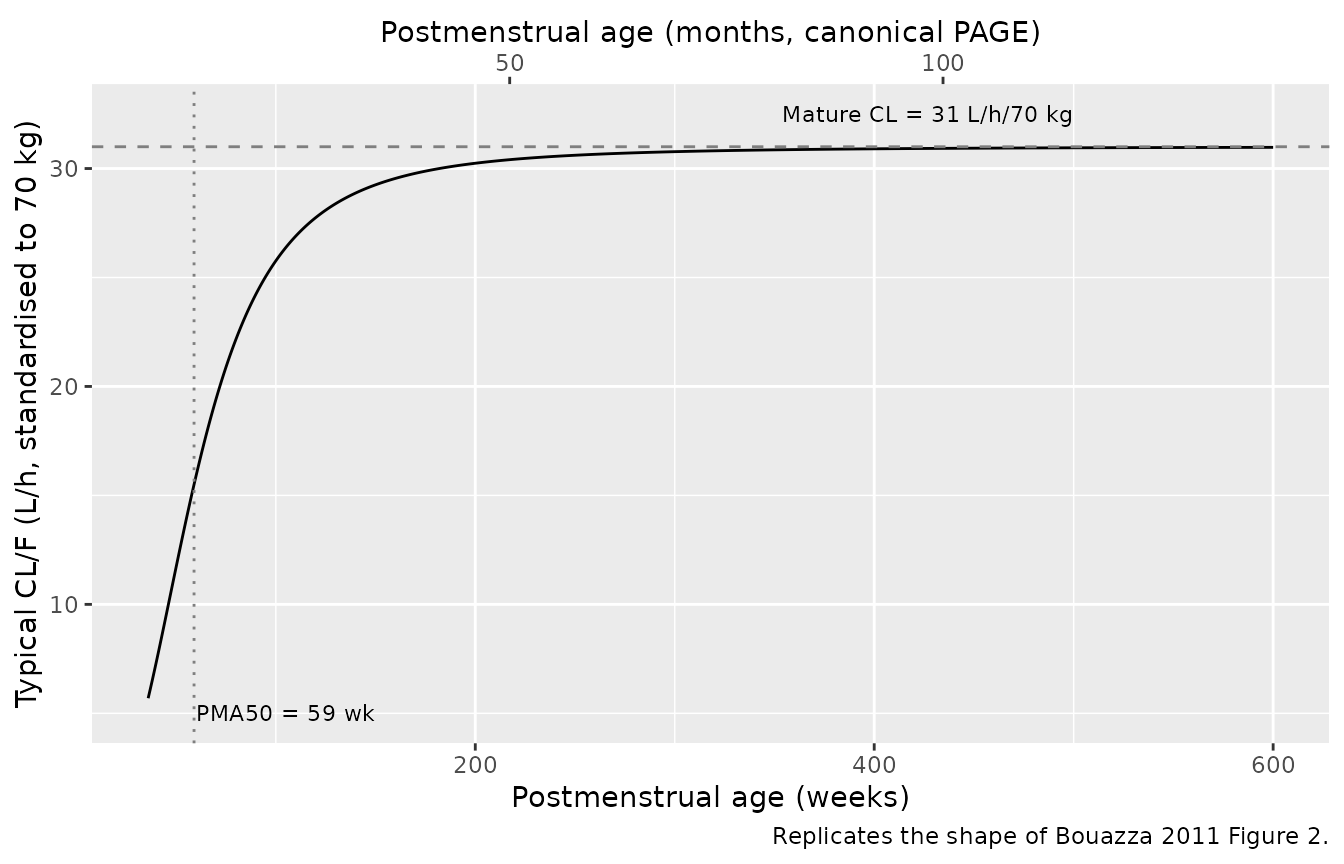
Virtual cohorts
Original observed data are not publicly available. The cohorts below match the four age strata from Bouazza 2011 Table 3 (Newborns, Infants, Children, Adolescents). For each stratum a single typical-value subject is simulated to steady state under the paper’s “FDA dosing” regimens; this is enough to reproduce the per-stratum apparent CL/F and AUC0-24 reported in Table 3 and the Table 2 BID/OAD comparison.
make_cohort <- function(label, wt_kg, page_months, dose_mg, tau_h,
                        ndoses, id) {
  # PAGE is the canonical postmenstrual-age column (months).
  # Use explicit per-dose rows (no addl) so PKNCA sees every dose event in
  # the steady-state interval used for the NCA below.
  dose_times <- seq(0, tau_h * (ndoses - 1L), by = tau_h)
  obs_grid   <- seq(0, tau_h * ndoses, by = 0.25)
  ev <- rxode2::et(amt = dose_mg, time = dose_times, cmt = "depot") |>
    rxode2::et(obs_grid)
  df <- as.data.frame(ev)
  df$id        <- id
  df$WT        <- wt_kg
  df$PAGE      <- page_months
  df$cohort    <- label
  df$regimen   <- if (tau_h == 12) "BID" else "OAD"
  df$dose_mg   <- dose_mg
  df
}

# PAGE for each age stratum (postmenstrual age in months; GA defaulted to term = 40 weeks)
# PNA stratum-median -> PAGE = (40 + 7*PNA_wk_each_kid)/4.345  (we just pick a typical PNA).
cohorts <- dplyr::bind_rows(
  # FDA regimen for newborns/infants: 4 mg/kg/day split BID
  make_cohort("Newborn (<1 mo)",      wt_kg = 3.5,  page_months = 9.67,  dose_mg = 7,    tau_h = 12, ndoses = 16, id =  1L),
  make_cohort("Infant (1-12 mo)",     wt_kg = 7,    page_months = 14.7,  dose_mg = 28,   tau_h = 12, ndoses = 16, id =  2L),
  # Older children: 8 mg/kg/day split BID
  make_cohort("Child (1-11 yr) BID",  wt_kg = 20,   page_months = 75.2,  dose_mg = 80,   tau_h = 12, ndoses = 16, id =  3L),
  make_cohort("Child (1-11 yr) OAD",  wt_kg = 20,   page_months = 75.2,  dose_mg = 160,  tau_h = 24, ndoses =  8, id =  4L),
  # Adolescents: 150 mg BID or 300 mg OAD per Table 2
  make_cohort("Adolescent BID",       wt_kg = 50,   page_months = 183.2, dose_mg = 150,  tau_h = 12, ndoses = 16, id =  5L),
  make_cohort("Adolescent OAD",       wt_kg = 50,   page_months = 183.2, dose_mg = 300,  tau_h = 24, ndoses =  8, id =  6L)
)

stopifnot(!anyDuplicated(unique(cohorts[, c("id", "time", "evid")])))
Simulation
Typical-value simulation (random effects zeroed) reproduces the cohort-median behaviour reported in Tables 2 and 3.
mod          <- rxode2::rxode(readModelDb("Bouazza_2011_lamivudine"))
#> ℹ parameter labels from comments will be replaced by 'label()'
mod_typical  <- rxode2::zeroRe(mod)
sim          <- rxode2::rxSolve(
  mod_typical, events = cohorts,
  keep = c("cohort", "regimen", "WT", "dose_mg")
) |>
  as.data.frame()
#> ℹ omega/sigma items treated as zero: 'etalcl', 'etalvc'
#> Warning: multi-subject simulation without without 'omega'
Concentration-time profiles
sim |>
  dplyr::filter(time >= max(time) - 24) |>            # one steady-state interval (last 24 h)
  dplyr::mutate(t_in_interval = time - (max(time) - 24)) |>
  ggplot(aes(t_in_interval, Cc, colour = regimen)) +
  geom_line(linewidth = 0.7) +
  facet_wrap(~ cohort, scales = "free_y") +
  scale_y_log10() +
  labs(x = "Time within steady-state 24-h interval (h)",
       y = "Plasma lamivudine (mg/L)",
       title = "Steady-state typical-value lamivudine profiles by cohort",
       caption = "Cohorts span Table 3 strata; BID and OAD regimens for adolescents and children per Table 2.")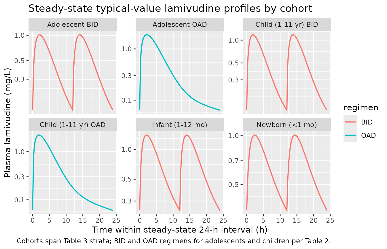
Replicates Table 3 (CL/F by age stratum)
Bouazza 2011 Table 3 reports median apparent CL/F in L/h/kg by age stratum. The table below reproduces the typical-value CL/F derived from the packaged model parameters at the cohort-median weight and PMA.
typical_cl <- tibble::tribble(
  ~cohort,                 ~WT, ~page_months,
  "Newborn (<1 mo)",       3.5,    9.67,
  "Infant (1-12 mo)",      7,     14.7,
  "Child (1-11 yr) BID",   20,    75.2,
  "Child (1-11 yr) OAD",   20,    75.2,
  "Adolescent BID",        50,   183.2,
  "Adolescent OAD",        50,   183.2
) |>
  dplyr::mutate(
    pma_wk       = page_months * 4.345,
    mat          = pma_wk^3.02 / (59^3.02 + pma_wk^3.02),
    cl_total_L_h = 31 * (WT / 70)^0.75 * mat,
    cl_kg        = cl_total_L_h / WT
  )

paper_cl <- tibble::tribble(
  ~cohort,                ~paper_dose_mg_kg_day, ~paper_cl_L_h_kg,
  "Newborn (<1 mo)",      4,                     0.26,
  "Infant (1-12 mo)",     7,                     0.49,
  "Child (1-11 yr) BID",  7.7,                   0.64,
  "Child (1-11 yr) OAD",  7.7,                   0.64,
  "Adolescent BID",       6.7,                   0.49,
  "Adolescent OAD",       6.7,                   0.49
)

dplyr::left_join(typical_cl, paper_cl, by = "cohort") |>
  dplyr::transmute(cohort, WT, page_months,
                   model_cl_L_h = round(cl_total_L_h, 2),
                   model_cl_L_h_kg = round(cl_kg, 3),
                   paper_cl_L_h_kg) |>
knitr::kable(caption = "Typical model CL/F vs. Bouazza 2011 Table 3 median CL/F (L/h/kg).")| cohort | WT | page_months | model_cl_L_h | model_cl_L_h_kg | paper_cl_L_h_kg |
|---|---|---|---|---|---|
| Newborn (<1 mo) | 3.5 | 9.67 | 0.87 | 0.247 | 0.26 |
| Infant (1-12 mo) | 7.0 | 14.70 | 3.08 | 0.441 | 0.49 |
| Child (1-11 yr) BID | 20.0 | 75.20 | 12.05 | 0.602 | 0.64 |
| Child (1-11 yr) OAD | 20.0 | 75.20 | 12.05 | 0.602 | 0.64 |
| Adolescent BID | 50.0 | 183.20 | 24.08 | 0.482 | 0.49 |
| Adolescent OAD | 50.0 | 183.20 | 24.08 | 0.482 | 0.49 |
PKNCA validation at steady state (replicates Table 2)
Bouazza 2011 Table 2 compares AUC0-24, Cmin, and Cmax for BID vs. OAD regimens in children and adolescents. PKNCA is used to compute the same metrics from the simulated typical-value profiles over a single steady-state 24-hour interval.
sim_nca <- sim |>
  dplyr::filter(!is.na(Cc), time >= max(time) - 24) |>
  dplyr::select(id, time, Cc, cohort)

dose_df <- cohorts |>
  dplyr::filter(evid == 1, time >= max(time) - 24) |>
  dplyr::select(id, time, amt, cohort)

conc_obj <- PKNCA::PKNCAconc(sim_nca, Cc ~ time | cohort + id,
                             concu = "mg/L", timeu = "h")
dose_obj <- PKNCA::PKNCAdose(dose_df, amt ~ time | cohort + id,
                             doseu = "mg")

start_ss <- max(dose_df$time)
end_ss   <- start_ss + 24

intervals <- data.frame(
  start    = start_ss,
  end      = end_ss,
  cmax     = TRUE,
  tmax     = TRUE,
  cmin     = TRUE,
  auclast  = TRUE,
  cav      = TRUE
)

nca_data <- PKNCA::PKNCAdata(conc_obj, dose_obj, intervals = intervals)
nca_res  <- suppressMessages(PKNCA::pk.nca(nca_data))

nca_tab <- as.data.frame(nca_res$result) |>
  dplyr::select(cohort, PPTESTCD, PPORRES) |>
  tidyr::pivot_wider(names_from = PPTESTCD, values_from = PPORRES) |>
  dplyr::transmute(
    cohort,
    sim_cmax_mg_L  = round(cmax, 2),
    sim_cmin_mg_L  = round(cmin, 3),
    sim_auclast_24 = round(auclast, 1)
  )

paper_tab <- tibble::tribble(
  ~cohort,                 ~paper_auc_0_24, ~paper_cmin_mg_L, ~paper_cmax_mg_L,
  "Child (1-11 yr) BID",   12.5,            0.11,             1.10,
  "Child (1-11 yr) OAD",   11.1,            0.05,             1.90,
  "Adolescent BID",        14.8,            0.15,             1.20,
  "Adolescent OAD",        12.8,            0.07,             1.90
)

dplyr::left_join(nca_tab, paper_tab, by = "cohort") |>
knitr::kable(caption = "Simulated typical-value steady-state NCA vs. Bouazza 2011 Table 2 medians. The two pediatric < 1 yr cohorts (Newborn, Infant) are not in Table 2 and do not have paper values for comparison.")| cohort | sim_cmax_mg_L | sim_cmin_mg_L | sim_auclast_24 | paper_auc_0_24 | paper_cmin_mg_L | paper_cmax_mg_L |
|---|---|---|---|---|---|---|
| Adolescent BID | 1.01 | 0.128 | 6.2 | 14.8 | 0.15 | 1.2 |
| Adolescent OAD | 0.19 | 0.063 | 1.2 | 12.8 | 0.07 | 1.9 |
| Child (1-11 yr) BID | 1.17 | 0.120 | 6.6 | 12.5 | 0.11 | 1.1 |
| Child (1-11 yr) OAD | 0.18 | 0.060 | 1.2 | 11.1 | 0.05 | 1.9 |
| Infant (1-12 mo) | 1.40 | 0.241 | 9.1 | NA | NA | NA |
| Newborn (<1 mo) | 1.01 | 0.346 | 8.1 | NA | NA | NA |
Assumptions and deviations
-
Allometric exponents fixed at 0.75 and 1. The paper
writes: “from allometric scaling theory these are typically 0.75 for
clearance parameters and 1 for volumes of distribution.” The exponents
are not in the Table 1 RSE listing, so they are encoded as
fixed()inini()– they represent the standard theoretical values used during fitting rather than parameters estimated from the data. -
Postmenstrual age in months (canonical PAGE) vs. weeks
(paper PMA). The canonical
PAGEcovariate column carries postmenstrual age in months; the paper’s PMA50 (59 weeks) and Hill exponent (3.02) are in weeks. The model() block multiplies PAGE by 4.345 (weeks per month) to evaluate the maturation function on the published scale without re-parameterising. -
Gestational-age imputation when missing. The paper
imputes GA = 40 weeks (term birth) when not reported. Downstream users
supplying PAGE directly should compute PAGE from
(GA_weeks + PNA_weeks) / 4.345; for a term newborn at age 0 this equals 9.20 months. -
Galenic form (tablet vs. solution). Tested and not
retained in the final model. Recorded in
covariatesDataExcludedso the screen is documented but is not represented inmodel(). - No IIV on Ka, Q, or Vp. Per Bouazza 2011 Results, IIV was retained only for CL/F and Vc/F; the other random effects were not significant.
- Vc/F IIV is large (omega = 0.77, ~90% CV). The paper reports eta-shrinkage of 0.39 (~39%) for Vc/F, exceeding the 25% threshold cited in the discussion; individual Vc/F EBEs are noisy but typical-value predictions are unaffected.
- Cohort cohort-medians for validation. The replication of Tables 2 and 3 uses one typical-value subject per cohort at the cohort-median WT and a representative PAGE. This is sufficient to recover the median CL/F per stratum and the BID/OAD AUC0-24, Cmax, Cmin medians. A full simulated VPC with between-subject variability is not in scope of this validation vignette.