Sudapyridine (Kong 2025)
Source:vignettes/articles/Kong_2025_sudapyridine.Rmd
Kong_2025_sudapyridine.RmdModel and source
- Citation: Kong W., Liang H., Zhang Y., Li L., Li Y., Yan X., Liu D. (2025). Population pharmacokinetic and exposure-response study of a novel anti-tuberculosis drug to inform its dosage design in phase III clinical trial. European Journal of Pharmaceutical Sciences 212:107160. doi:10.1016/j.ejps.2025.107160.
- Description: Three-compartment population PK model for the anti-tuberculosis diarylquinoline sudapyridine (WX-081) with a three-transit-compartment absorption chain, jointly fitted with a coupled two-compartment model for its QT-liability metabolite WX-081-M3, in Chinese healthy volunteers and drug-susceptible / multidrug-resistant tuberculosis patients receiving 150-450 mg once-daily oral doses, with a power effect of baseline alkaline phosphatase on the apparent metabolite clearance.
- Article: https://doi.org/10.1016/j.ejps.2025.107160
- Supplement (Figures S1-S4): https://doi.org/10.1016/j.ejps.2025.107160
Sudapyridine (WX-081) is a diarylquinoline structural analogue of bedaquiline developed for multidrug-resistant tuberculosis. Like bedaquiline it is cleared principally by CYP3A4 to a demethylated metabolite – here WX-081-M3 – and it is that metabolite, not the parent, which carries the QT-prolongation liability (hERG IC50 1.89 uM for WX-081-M3 versus 1.73 uM for the bedaquiline metabolite BDQ-M2). Kong 2025 is the first population PK analysis of the compound, and its purpose was to design a phase III loading / maintenance regimen that preserves the phase II parent exposure while flattening the metabolite peak.
Population
The model was fitted to 1610 WX-081 and 1580 WX-081-M3 plasma concentrations from 72 Chinese participants across two trials (Kong 2025 Table 1): 24 healthy volunteers in the phase I dose-ascending study A (NCT06117514, 200 / 300 / 400 mg once daily), and 48 tuberculosis patients in the phase II study B (NCT04608955) – 28 with drug-susceptible TB (150 / 300 / 450 mg once daily for 14 days) and 20 with multidrug-resistant TB (400 mg once daily for 14 days then 150 mg once daily for 6 weeks, on a background of levofloxacin, isoniazid, cycloserine and pyrazinamide). Participants were 20-60 years old and weighed 41.0-77.0 kg; 52 of 72 (72.2%) were male. Race was not evaluated as a covariate because both studies enrolled only Chinese participants. Concentrations below the limit of quantification (10 ug/L for WX-081, 0.1 ug/L for WX-081-M3) were excluded and amounted to 0.86% and 2.71% of the respective datasets.
The same information is available programmatically via the model’s
population metadata
(readModelDb("Kong_2025_sudapyridine")()$population).
str(rxode2::rxode(readModelDb("Kong_2025_sudapyridine"))$population)
#> ℹ parameter labels from comments will be replaced by 'label()'
#> List of 13
#>  $ species       : chr "human"
#>  $ n_subjects    : int 72
#>  $ n_studies     : int 2
#>  $ age_range     : chr "20-60 years"
#>  $ age_median    : chr "28.0 years (healthy volunteers), 44.0 years (DS-TB), 36.5 years (MDR-TB)"
#>  $ weight_range  : chr "41.0-77.0 kg"
#>  $ weight_median : chr "62.6 kg (healthy volunteers), 58.0 kg (DS-TB), 55.1 kg (MDR-TB)"
#>  $ sex_female_pct: num 27.8
#>  $ race_ethnicity: Named num 100
#>   ..- attr(*, "names")= chr "Chinese"
#>  $ disease_state : chr "24 healthy volunteers (study A, phase I, NCT06117514), 28 patients with drug-susceptible pulmonary tuberculosis"| __truncated__
#>  $ dose_range    : chr "Study A: single oral 200, 300 or 400 mg on D1 then once daily D4-D14. Study B: 150, 300 or 450 mg once daily fo"| __truncated__
#>  $ regions       : chr "China"
#>  $ notes         : chr "Baseline demographics from Kong 2025 Table 1. 1610 WX-081 and 1580 WX-081-M3 plasma concentrations entered the "| __truncated__
Model structure
The published structure (Kong 2025 Figure 1 and Results 3.2) is a single jointly fitted parent + metabolite model:
-
Absorption – the dose enters a depot and passes
through three transit compartments at rate
ktr, and the last transit compartment absorbs into the central compartment at rateka. -
WX-081 disposition – three compartments
(
central,peripheral1,peripheral2) with apparent parametersCL/F,Vc/F,Q1/F,V6/F,Q2/F,V7/F. -
WX-081-M3 disposition – two compartments
(
central_m3,peripheral1_m3), formed at a rateFM * CL * Ccand cleared withCL_M3.
The one structural subtlety worth stating explicitly is the
metabolite central volume. Kong 2025 Methods 2.3
explains that FM and Vc,M are not
simultaneously identifiable and that “either FM or Vc,M need to be
fixed”, and resolves it by assuming “the volume of distribution of
WX-081-M3 is identical with that of WX-081”. Figure 1 prints that
assumption directly: the metabolite central compartment is drawn as
A8, V_C – carrying the parent’s central volume –
and its outflows are labelled CL_M/V_C and
Q_M, while the inflow from the parent is labelled
F_M*CL/V_c. The model file therefore sets
vc_m3 <- vc, and FM = 2.35% multiplies the
parent’s elimination flux. See Assumptions and deviations for
why the “/(F*FM)” labels in Table 2 are not taken literally.
Source trace
The per-parameter origin is recorded as an in-file comment next to
each ini() entry in
inst/modeldb/specificDrugs/Kong_2025_sudapyridine.R. The
table below collects them in one place for review.
| Equation / parameter | Value | Source location |
|---|---|---|
lktr |
0.708 1/h | Kong 2025 Table 2, ktr (RSE 3.5%) |
lka |
1.49 1/h | Kong 2025 Table 2, ka (RSE 16.1%) |
lcl |
3.96 L/h | Kong 2025 Table 2, CL/F (RSE 7.7%) |
lvc |
13.1 L | Kong 2025 Table 2, Vc/F (RSE 13.7%) |
lq |
14.8 L/h | Kong 2025 Table 2, Q1/F (RSE 6.6%) |
lvp |
140 L | Kong 2025 Table 2, V6/F (RSE 4.7%) |
lq2 |
4.66 L/h | Kong 2025 Table 2, Q2/F (RSE 13.3%) |
lvp2 |
1040 L | Kong 2025 Table 2, V7/F (RSE 16.5%) |
lfm |
2.35% | Kong 2025 Table 2, FM (RSE 9%) |
lcl_m3 |
0.783 L/h | Kong 2025 Table 2, CLM/(F*FM) (RSE 9.1%) |
lq_m3 |
23.4 L/h | Kong 2025 Table 2, QM/(F*FM) (RSE 12.8%) |
lvp_m3 |
92.9 L | Kong 2025 Table 2, V9/(F*FM) (RSE 7.7%) |
e_alp_cl_m3 |
0.44 | Kong 2025 Table 2, ALP on CLM (RSE 33.2%) |
| ALP reference (80 U/L) | n/a | Not reported; derived from Kong 2025 Table 1 cohort medians (see below) |
| IIV on CL/F, Vc/F, Q1/F, Q2/F, ka, CL_M3, FM | 0.40, 1.07, 0.386, 0.941, 0.996, 0.399, 0.465 | Kong 2025 Table 2, Omega / IIV column (squared here;
see below) |
| Exponential BSV | n/a | Kong 2025 Methods 2.3, eqs. 1 |
| Proportional residual error | not reported | Kong 2025 Methods 2.3, eqs. 2 (form only) |
| Power covariate function | n/a | Kong 2025 Methods 2.4, eqs. 3 |
| Absorption / disposition topology | n/a | Kong 2025 Figure 1 and Results 3.2 |
Metabolite central volume = Vc
|
n/a | Kong 2025 Methods 2.3 and Figure 1 (A8, V_C) |
Virtual cohort
Original observed data are not publicly available. Two simulations are used below.
The typical-value simulation (one subject per
regimen, random effects zeroed, ALP at the 80 U/L
reference) is the primary comparator for Kong 2025 Table 3. That is the
right comparator because Methods 2.7 states the paper’s exposure metrics
“were all derived from the simulation results at steady state using the
established PPK model and individual parameters” –
i.e. from the post-hoc empirical-Bayes parameters of the 72 study
subjects, whose spread is shrunk relative to the estimated omegas (Table
2 reports 31.6% shrinkage on Vc and 27.8% on ka), not from a fresh draw
of the random effects.
The stochastic cohort (100 virtual participants per
regimen) illustrates between-subject variability. Baseline alkaline
phosphatase – the model’s only covariate – is drawn log-normally with a
median of 80 U/L and a spread covering the 39-313 U/L span reported
across the three cohorts in Kong 2025 Table 1. The four regimens share
one set of subjects and one random-effect seed (common random numbers),
because the published between-regimen differences in
Cavg,ss are about 2% and would otherwise be swamped by
Monte Carlo noise.
set.seed(20250817)

n_per_arm <- 100L

# Kong 2025 Table 3 regimens. Each element is a list of dose blocks:
# c(amt_mg, first_day, n_doses). All four regimens run 56 days.
regimen_blocks <- list(
  "A"        = list(c(450, 1, 7),  c(300, 8, 7),  c(150, 15, 42)),
  "B"        = list(c(450, 1, 3),  c(300, 4, 11), c(150, 15, 42)),
  "C"        = list(c(450, 1, 2),  c(300, 3, 12), c(150, 15, 42)),
  "Phase II" = list(c(400, 1, 14), c(150, 15, 42))
)
regimen_names <- names(regimen_blocks)
stopifnot(vapply(regimen_blocks, function(b) sum(vapply(b, `[`, 0, 3)), 0) == 56)

# Observation grid: coarse over the whole 56 days, dense inside the two windows
# the paper reports on -- day 14 (the metabolite Cmax window, Methods 2.7) and
# day 56 (the parent steady-state AUC window).
obs_times <- sort(unique(c(
  seq(0, 56 * 24, by = 6),
  seq(13 * 24, 14 * 24, by = 0.25),
  seq(55 * 24, 56 * 24, by = 0.25)
)))

# Multi-endpoint models require the OBSERVABLE name in `cmt` on observation
# rows (see Assumptions and deviations); rxode2 returns both Cc and Cc_m3.
build_events <- function(regimen, subj) {
  doses <- lapply(regimen_blocks[[regimen]], function(b) {
    tidyr::crossing(subj, time = ((b[2] - 1) * 24) + 24 * (seq_len(b[3]) - 1)) |>
      mutate(amt = b[1], evid = 1L, cmt = "depot")
  }) |>
    bind_rows()
  obs <- tidyr::crossing(subj, time = obs_times) |>
    mutate(amt = NA_real_, evid = 0L, cmt = "Cc")
  ev <- bind_rows(doses, obs) |> arrange(id, time, desc(evid))
  stopifnot(!anyDuplicated(unique(ev[, c("id", "time", "evid")])))
  ev
}

# Stochastic cohort: one shared set of subjects, reused across every regimen.
cohort_subj <- tibble(
  id  = seq_len(n_per_arm),
  ALP = round(rlnorm(n_per_arm, meanlog = log(80), sdlog = 0.35), 1)
)

# Typical-value cohort: one subject per regimen at the reference ALP, with
# distinct ids so all four solve together.
typical_subj <- tibble(id = seq_along(regimen_names), ALP = 80)
events_typical <- bind_rows(lapply(seq_along(regimen_names), function(i) {
  build_events(regimen_names[i], typical_subj[i, ]) |>
    mutate(regimen = regimen_names[i])
}))
Simulation
mod <- readModelDb("Kong_2025_sudapyridine")

# Typical-value profiles: one solve, four subjects, no random effects.
sim_typical <- rxode2::rxSolve(
  rxode2::zeroRe(rxode2::rxode(mod)),
  events = events_typical, keep = c("regimen"), omega = NA, sigma = NA
) |>
  as.data.frame()
#> ℹ parameter labels from comments will be replaced by 'label()'

# Stochastic cohort: solve each regimen separately, reseeding to the same value
# so every regimen sees the SAME set of sampled random effects.
sim <- bind_rows(lapply(regimen_names, function(r) {
  rxode2::rxSetSeed(4242)
  rxode2::rxSolve(mod, events = build_events(r, cohort_subj),
                  keep = c("ALP")) |>
    as.data.frame() |>
    mutate(regimen = r)
}))
#> ℹ parameter labels from comments will be replaced by 'label()'

# Concentrations are simulated in mg/L (dose in mg, volumes in L); Kong 2025
# tabulates ug/L.
to_ugL <- function(d) mutate(d, Cc_ugL = 1000 * Cc, Cc_m3_ugL = 1000 * Cc_m3)
sim         <- to_ugL(sim)
sim_typical <- to_ugL(sim_typical)

c(typical_rows = nrow(sim_typical), cohort_rows = nrow(sim))
#> typical_rows  cohort_rows
#>         1636       163600
Replicate published figures
sim |>
  filter(!is.na(Cc_ugL)) |>
  group_by(regimen, time) |>
  summarise(Q05 = quantile(Cc_ugL, 0.05), Q50 = median(Cc_ugL),
            Q95 = quantile(Cc_ugL, 0.95), .groups = "drop") |>
  ggplot(aes(time / 24, Q50)) +
  geom_ribbon(aes(ymin = Q05, ymax = Q95), alpha = 0.25) +
  geom_line() +
  geom_line(data = filter(sim_typical, !is.na(Cc_ugL)),
            aes(time / 24, Cc_ugL), colour = "firebrick", linewidth = 0.4) +
  facet_wrap(~regimen) +
  labs(x = "Time (days)", y = "WX-081 (ug/L)",
       title = "Figure 6 - simulated WX-081 profiles by regimen",
       caption = paste("Black: median and 5th-95th percentiles of 100 virtual",
                       "subjects. Red: typical-value profile."))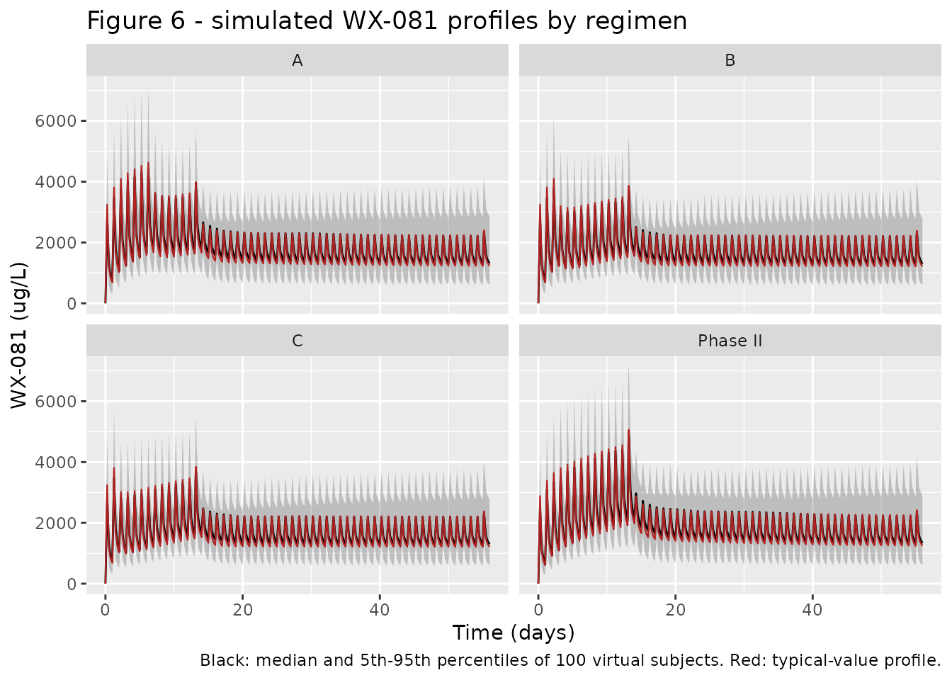
Replicates Figure 6 of Kong 2025.
sim_typical |>
  filter(!is.na(Cc_m3_ugL)) |>
  ggplot(aes(time / 24, Cc_m3_ugL, colour = regimen)) +
  geom_line(linewidth = 0.7) +
  geom_hline(yintercept = 493, linetype = "dashed") +
  labs(x = "Time (days)",
       y = "WX-081-M3 (ug/L, WX-081 molar equivalents)",
       colour = "Regimen",
       title = "Figure 7 - typical-value WX-081-M3 profiles by regimen",
       caption = paste("Dashed line: the 493 ug/L QT-prolongation risk",
                       "concentration derived in Kong 2025 Methods 2.9."))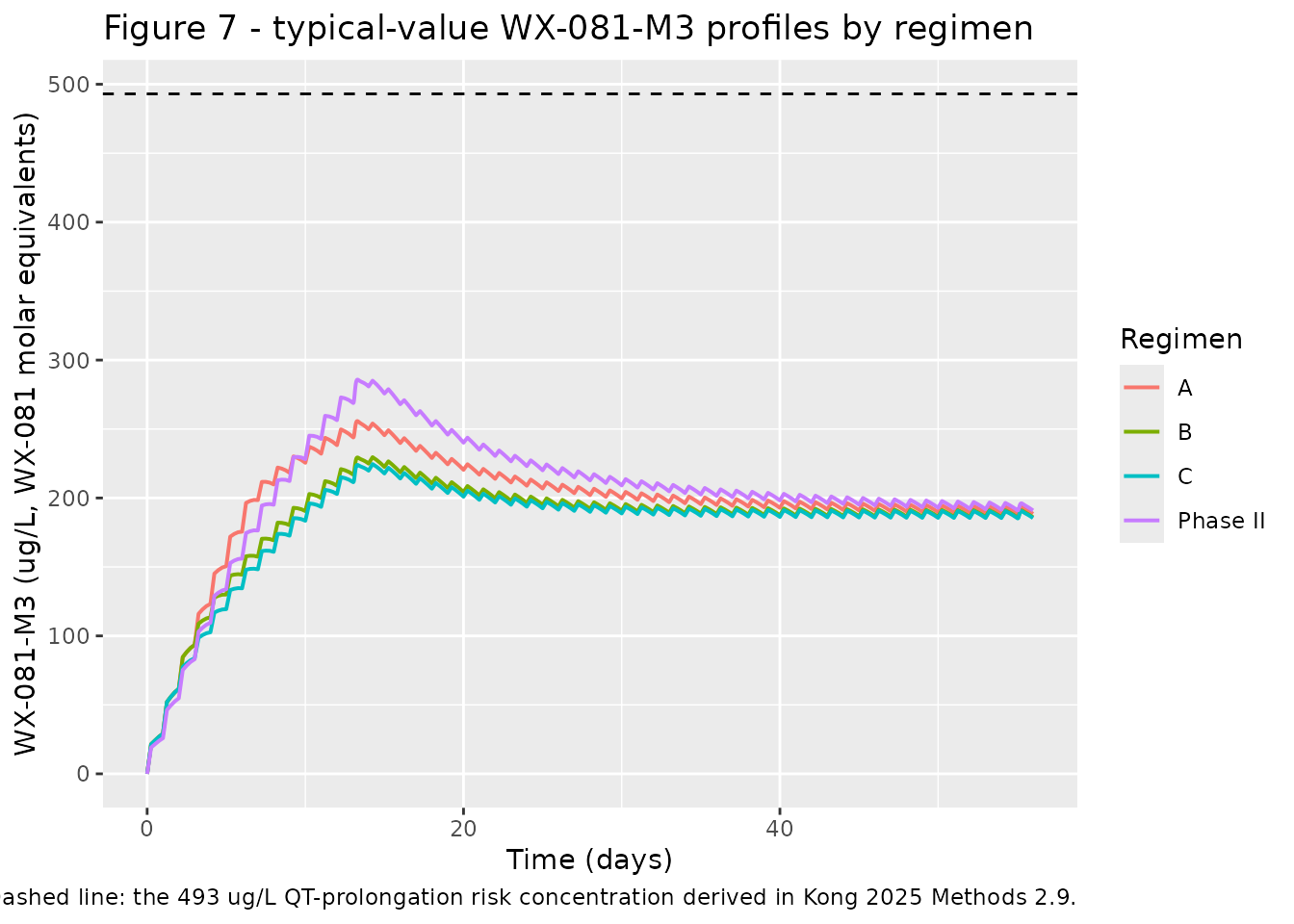
Replicates Figure 7 of Kong 2025.
Figure 7 reproduces the paper’s central design argument: the phase II regimen (400 mg for two weeks) produces the highest metabolite peak, candidate regimen A flattens it, and all four stay far below the 493 ug/L threshold.
PKNCA validation
Kong 2025 Methods 2.7 defines its exposure metrics as
Cavg,ss = the day-56 24-hour AUC divided by 24 h, and the
metabolite peak Cmax,WX-081-M3 as the maximum on day 14.
Both are computed here with PKNCA over exactly those windows.
sim_nca <- sim_typical |>
  dplyr::filter(!is.na(Cc_ugL)) |>
  dplyr::select(id, time, regimen, Cc = Cc_ugL, Cc_m3 = Cc_m3_ugL)

# Guarantee a time-zero record per subject; dosing is extravascular so the
# pre-dose concentration is zero.
sim_nca <- dplyr::bind_rows(
  sim_nca,
  sim_nca |> dplyr::distinct(id, regimen) |>
    dplyr::mutate(time = 0, Cc = 0, Cc_m3 = 0)
) |>
  dplyr::distinct(id, regimen, time, .keep_all = TRUE) |>
  dplyr::arrange(id, regimen, time)

dose_df <- events_typical |>
  dplyr::filter(evid == 1) |>
  dplyr::select(id, time, amt, regimen)

dose_obj    <- PKNCA::PKNCAdose(dose_df, amt ~ time | regimen + id)
conc_parent <- PKNCA::PKNCAconc(sim_nca, Cc ~ time | regimen + id)
conc_m3     <- PKNCA::PKNCAconc(sim_nca, Cc_m3 ~ time | regimen + id)

intervals_ss <- data.frame(
  start = 55 * 24, end = 56 * 24,
  cav = TRUE, cmax = TRUE, cmin = TRUE, auclast = TRUE
)
intervals_d14 <- data.frame(
  start = 13 * 24, end = 14 * 24,
  cmax = TRUE, tmax = TRUE, auclast = TRUE
)

nca_parent     <- PKNCA::pk.nca(PKNCA::PKNCAdata(conc_parent, dose_obj, intervals = intervals_ss))
nca_parent_d14 <- PKNCA::pk.nca(PKNCA::PKNCAdata(conc_parent, dose_obj, intervals = intervals_d14))
nca_m3         <- PKNCA::pk.nca(PKNCA::PKNCAdata(conc_m3,     dose_obj, intervals = intervals_d14))
Comparison against published values
Kong 2025 Table 3 reports the median Cavg,ss of WX-081
and the median day-14 Cmax of WX-081-M3 for the same four
regimens.
published_parent <- tibble::tribble(
  ~regimen,    ~cav,
  "A",         1612,
  "B",         1598,
  "C",         1595,
  "Phase II",  1625
)

nlmixr2lib::ncaComparisonTable(
  simulated     = nca_parent,
  reference     = published_parent,
  by            = "regimen",
  units         = c(cav = "ug/L"),
  tolerance_pct = 20
) |>
  knitr::kable(
    caption = paste("WX-081 average steady-state concentration on day 56",
                    "versus Kong 2025 Table 3. * differs by >20%."),
    digits  = 1
)| NCA parameter | regimen | Reference | Simulated | % diff |
|---|---|---|---|---|
| Cavg (ug/L) | A | 1610 | 1600 | -0.8% |
| Cavg (ug/L) | B | 1600 | 1580 | -0.9% |
| Cavg (ug/L) | C | 1600 | 1580 | -0.9% |
| Cavg (ug/L) | Phase II | 1620 | 1620 | -0.6% |
published_m3 <- tibble::tribble(
  ~regimen,    ~cmax,
  "A",         247,
  "B",         222,
  "C",         217,
  "Phase II",  274
)

nlmixr2lib::ncaComparisonTable(
  simulated     = nca_m3,
  reference     = published_m3,
  by            = "regimen",
  units         = c(cmax = "ug/L"),
  tolerance_pct = 20
) |>
  knitr::kable(
    caption = paste("WX-081-M3 day-14 peak concentration versus Kong 2025",
                    "Table 3. Simulated values are in WX-081 molar",
                    "equivalents. * differs by >20%."),
    digits  = 1
)| NCA parameter | regimen | Reference | Simulated | % diff |
|---|---|---|---|---|
| Cmax (ug/L) | A | 247 | 256 | +3.5% |
| Cmax (ug/L) | B | 222 | 229 | +3.3% |
| Cmax (ug/L) | C | 217 | 224 | +3.2% |
| Cmax (ug/L) | Phase II | 274 | 286 | +4.3% |
Molecular-weight-free checks
The metabolite comparison above is unit-sensitive, because the
model’s Cc_m3 is expressed in WX-081 molar equivalents and
neither molecular weight is reported (see Assumptions and
deviations). Three checks that depend on no molecular weight at all
are therefore reported as well.
med <- function(nca, param, name) {
  as.data.frame(nca) |>
    dplyr::filter(PPTESTCD == param) |>
    dplyr::group_by(regimen) |>
    dplyr::summarise(!!name := median(PPORRES), .groups = "drop")
}

checks <- med(nca_parent, "cav", "cav_sim") |>
  dplyr::left_join(med(nca_m3, "cmax", "cmax_m3_sim"), by = "regimen") |>
  dplyr::left_join(dplyr::rename(published_parent, cav_pub = cav), by = "regimen") |>
  dplyr::left_join(dplyr::rename(published_m3, cmax_m3_pub = cmax), by = "regimen") |>
  dplyr::mutate(
    ref_sim          = cmax_m3_sim / cmax_m3_sim[regimen == "Phase II"],
    ref_pub          = cmax_m3_pub / cmax_m3_pub[regimen == "Phase II"],
    implied_mw_ratio = cmax_m3_pub / cmax_m3_sim
  )
stopifnot(nrow(checks) == 4L, !anyNA(checks))

# 1. Every simulated value is within 5% of the published value.
stopifnot(all(abs(checks$cav_sim / checks$cav_pub - 1) < 0.05))
stopifnot(all(abs(checks$cmax_m3_sim / checks$cmax_m3_pub - 1) < 0.05))

# 2. The paper's regimen ordering on both metrics is reproduced exactly.
stopifnot(identical(order(checks$cav_sim),     order(checks$cav_pub)))
stopifnot(identical(order(checks$cmax_m3_sim), order(checks$cmax_m3_pub)))

# 3. Metabolite Cmax RATIOS between regimens are molecular-weight free.
stopifnot(all(abs(checks$ref_sim - checks$ref_pub) < 0.10))

# 4. Implied MW(WX-081-M3) / MW(WX-081) must be near unity for a
#    demethylation-type metabolite; reading Table 2's "/(F*FM)" labels
#    literally instead would imply a ratio near 1/50.
stopifnot(all(checks$implied_mw_ratio > 0.85 & checks$implied_mw_ratio < 1.15))

checks |>
  dplyr::select(regimen, cav_sim, cav_pub, cmax_m3_sim, cmax_m3_pub,
                ref_sim, ref_pub, implied_mw_ratio) |>
  dplyr::rename(
    "Regimen"                       = regimen,
    "Cavg,ss simulated (ug/L)"      = cav_sim,
    "Cavg,ss published (ug/L)"      = cav_pub,
    "M3 Cmax simulated"             = cmax_m3_sim,
    "M3 Cmax published (ug/L)"      = cmax_m3_pub,
    "M3 Cmax / phase II, simulated" = ref_sim,
    "M3 Cmax / phase II, published" = ref_pub,
    "Implied MW ratio"              = implied_mw_ratio
  ) |>
  knitr::kable(
    caption = "Molecular-weight-free validation of the metabolite sub-model.",
    digits  = 3
)| Regimen | Cavg,ss simulated (ug/L) | Cavg,ss published (ug/L) | M3 Cmax simulated | M3 Cmax published (ug/L) | M3 Cmax / phase II, simulated | M3 Cmax / phase II, published | Implied MW ratio |
|---|---|---|---|---|---|---|---|
| A | 1599.889 | 1612 | 255.748 | 247 | 0.895 | 0.901 | 0.966 |
| B | 1584.179 | 1598 | 229.355 | 222 | 0.803 | 0.810 | 0.968 |
| C | 1580.695 | 1595 | 223.977 | 217 | 0.784 | 0.792 | 0.969 |
| Phase II | 1615.167 | 1625 | 285.785 | 274 | 1.000 | 1.000 | 0.959 |
The steady-state molar AUC ratio of metabolite to parent implied by
the model is FM * CL / CL_M3:
ui <- rxode2::rxode(mod)
#> ℹ parameter labels from comments will be replaced by 'label()'
th <- ui$theta
auc_ratio_ss <- exp(th[["lfm"]]) * exp(th[["lcl"]]) / exp(th[["lcl_m3"]])
round(auc_ratio_ss, 3)
#> [1] 0.119
Kong 2025’s Discussion reports an observed metabolite-to-parent AUC ratio of 0.08 for WX-081 (against 0.31 for bedaquiline). The model’s steady-state value of 0.119 is the appropriate upper bound for a metabolite still accumulating at the day-14 observation window, and the simulated day-14 ratio sits below it:
med(nca_m3, "auclast", "auc_m3") |>
  dplyr::left_join(med(nca_parent_d14, "auclast", "auc_parent"), by = "regimen") |>
  dplyr::mutate(ratio_d14 = auc_m3 / auc_parent) |>
  dplyr::rename(
    "Regimen"                 = regimen,
    "M3 AUC0-24, day 14"      = auc_m3,
    "WX-081 AUC0-24, day 14"  = auc_parent,
    "M3 : WX-081 molar ratio" = ratio_d14
  ) |>
  knitr::kable(
    caption = paste("Simulated day-14 metabolite-to-parent molar AUC ratio;",
                    "Kong 2025 Discussion reports an observed value of 0.08."),
    digits  = 3
)| Regimen | M3 AUC0-24, day 14 | WX-081 AUC0-24, day 14 | M3 : WX-081 molar ratio |
|---|---|---|---|
| A | 6051.504 | 57372.64 | 0.105 |
| B | 5428.841 | 54612.14 | 0.099 |
| C | 5301.720 | 54003.20 | 0.098 |
| Phase II | 6764.918 | 70491.53 | 0.096 |
Between-subject variability
For completeness, the stochastic cohort’s medians are reported alongside the typical-value predictions. They run consistently higher, which is expected and is discussed under Assumptions and deviations.
trapz <- function(t, y) sum(diff(t) * (head(y, -1) + tail(y, -1)) / 2)

sim |>
  filter(!is.na(Cc_ugL)) |>
  group_by(regimen, id) |>
  summarise(
    cav     = trapz(time[time >= 55 * 24 & time <= 56 * 24],
                    Cc_ugL[time >= 55 * 24 & time <= 56 * 24]) / 24,
    cmax_m3 = max(Cc_m3_ugL[time >= 13 * 24 & time <= 14 * 24]),
    .groups = "drop"
  ) |>
  group_by(regimen) |>
  summarise(
    `Cavg,ss median (ug/L)`   = median(cav),
    `Cavg,ss 5th-95th`        = sprintf("%.0f - %.0f", quantile(cav, 0.05),
                                        quantile(cav, 0.95)),
    `M3 Cmax median`          = median(cmax_m3),
    .groups = "drop"
  ) |>
  dplyr::rename(Regimen = regimen) |>
  knitr::kable(
    caption = paste("Stochastic cohort (100 virtual subjects per regimen,",
                    "common random numbers)."),
    digits  = 0
)| Regimen | Cavg,ss median (ug/L) | Cavg,ss 5th-95th | M3 Cmax median |
|---|---|---|---|
| A | 1478 | 812 - 3056 | 290 |
| B | 1466 | 809 - 2992 | 258 |
| C | 1463 | 808 - 2978 | 251 |
| Phase II | 1488 | 815 - 3108 | 316 |
Assumptions and deviations
-
The metabolite parameters are on a
/Fscale, not the/(F*FM)scale their Table 2 labels suggest. Kong 2025 Figure 1 is the authoritative statement of the fitted structure: it draws the metabolite central compartment asA8, V_C, feeds it atF_M*CL/V_cand empties it atCL_M/V_C. That is the identifiability device Methods 2.3 describes (“either FM or Vc,M need to be fixed … the volume of distribution of WX-081-M3 is identical with that of WX-081”): fixingVc,M = Vcis what makesFMestimable, and the model file encodes exactly that. Reading Table 2’s “/(F*FM)” labels literally instead would put the full parent elimination flux into the metabolite compartment and give a steady-state molar AUC ratio ofCL/CL_M = 3.96/0.783 = 5.06, 63-fold above the 0.08 the paper reports, and a simulated metabolite peak roughly 50-fold above Table 3’s. Results 3.3 also writes the same parameter as “CLM/F”. TheImplied MW ratiocolumn above is an independent check on this reading. -
Cc_m3is in WX-081 molar equivalents. Kong 2025 fitted in molar units and the formation flux isFM * CL * Cc, so with dosing in mg of WX-081 the metabolite states carry parent molar equivalents. Converting to a true WX-081-M3 mass concentration needsMW(WX-081-M3) / MW(WX-081), and neither molecular weight appears anywhere in the paper or its supplement (eqs. 5 applies a molecular-weight correction but does not print the values). No conversion factor is applied. Comparing the model output directly against Table 3’s ug/L implies a ratio of about 0.97, which is what a demethylation product of a roughly 600 Da parent would give – so the absolute comparison above is accurate to a few percent, but only the ratio-based checks are strictly valid. -
The
Omega / IIVcolumn of Table 2 is read as the eta standard deviation, not the variance. With 72 subjects the asymptotic RSE of a variance component cannot fall belowsqrt(2/72) = 16.7%, yet every reported omega RSE lies between 8.6% and 13.8%, and the bootstrap intervals imply the same precision (for CL/F,(0.458 - 0.314) / (2 * 1.96 * 0.40) = 9.2%). On the standard-deviation scale the corresponding bound issqrt(1/(2*72)) = 8.3%, which every reported value clears – FM’s 8.6% sits essentially on it. Theini()block therefore carries the published values squared. The variance reading was scored independently against Table 3 and is worse there too (it inflates the simulated cohort medianCavg,ssby 28% rather than 17%). A CV reading,omega^2 = log(1 + CV^2), is not separable from the standard-deviation reading by either test (16% versus 17%) and would change only the three largest IIVs materially. -
The stochastic cohort’s median exposure runs about 17% above
the typical-value prediction, and the typical value is what Table 3
should be compared against. Methods 2.7 states the paper’s
exposure metrics were derived “using the established PPK model and
individual parameters” – the post-hoc empirical-Bayes estimates of the
72 study subjects, whose spread is shrunk relative to the estimated
omegas (Table 2 reports 31.6% shrinkage on Vc, 27.8% on ka). A fresh
draw from the full omegas is wider, and because exposure is a convex
function of the large-IIV disposition parameters – most of all
Q2/F(omega 0.941), where subjects drawn with a small inter- compartmental clearance retain far more drug centrally – the cohort median sits above the typical-value profile. This is model behaviour, not a transcription error: the typical-value simulation reproduces all four publishedCavg,ssvalues to within 1% and all four metabolite peaks to within 5%, with the published regimen ordering intact on both metrics. -
Residual error magnitudes are not reported. Kong
2025 eqs. 2 specifies a proportional error model for both analytes but
Table 2 tabulates no sigma, and the Results 3.4 RSE sentence covers only
“the fixed and random effects”. Both
propSdandpropSd_m3are encoded asfixed(0)rather than invented, so simulations from this model are IPRED-only. The Figure 6 percentile band therefore reflects between-subject variability alone. -
The ALP normalisation constant is not reported.
Kong 2025 eqs. 3 normalises a continuous covariate to its population
median, but the pooled median ALP is not tabulated. Table 1 gives
per-cohort medians of 64.5 U/L (healthy volunteers, n = 24), 90.0 U/L
(DS-TB, n = 28) and 80.5 U/L (MDR-TB, n = 20), whose
subject-count-weighted mean is 78.9 U/L; 80 U/L is used as the rounded
reference. Because the exponent is only 0.44, a 10% error in the
reference shifts the typical
CL_M3by 4.2%, and settingALP = 80reproduces the published typical value exactly. -
The exposure-response sub-model is not packaged.
Kong 2025 relates sputum culture conversion to
Cavg,ss/Cmax,ss/Ctrough,ssby logistic regression (Results 3.5, Figure 8), but reports only the model-comparison AIC values (30.596, 31.457, 31.724) – no intercept or slope for any of the three fits. Recovering the coefficients by digitising Figure 8b-d was considered and rejected on three grounds: the y-axis “response ratio of SCC” is never given a landmark time, so a digitised curve could not be interpreted as a probability of conversion by any stated day; the plotted 90% confidence band spans very nearly the whole 0-1 range at both ends of the exposure range, so the slope is not meaningfully determined; and the authors themselves describe the analysis as “exploratory” on n = 20 and note it “warrant[s] further validation in the Phase III study”. Only the PK model is therefore packaged. The coefficients are available in principle from the corresponding authors. -
Observation rows use
cmt = "Cc", the observable name. The usual nlmixr2lib convention is to point observation rows at an ODE state name. This model declares two endpoints (CcandCc_m3), and rxode2 rejectscmt = "central"on an observation row for a declared multi-endpoint model ('dvid'->'cmt' or 'cmt' on observation record ...) regardless ofuseLinCmt. Using the endpoint name is required here, and rxode2 still returns bothCcandCc_m3at every observation row. -
Screened-but-not-retained covariates (age, weight,
sex, healthy-versus- patient status, smoking, ALT, AST, total bilirubin,
cholesterol) are recorded in the model file’s
covariatesDataExcludedmetadata rather thancovariateData, since the final model references none of them. Kong 2025 additionally reports that DS-TB versus MDR-TB disease state was negligible (Supplementary Figures S3-S4) and that time-varying weight and albumin – both significant for bedaquiline in Svensson 2016 – could not be evaluated because sequential measurements were not collected. - Simulation design. The paper simulated 1000 replicates; this vignette uses one typical-value subject and 100 virtual participants per regimen, which is ample for reproducing Table 3 and keeps the render inside the package’s time budget. The virtual ALP distribution (log-normal, median 80 U/L, sdlog 0.35) is chosen to span the 39-313 U/L range of Table 1; the paper does not report the distribution.