Raltegravir (Gurjar 2023)
Source:vignettes/articles/Gurjar_2023_raltegravir.Rmd
Gurjar_2023_raltegravir.RmdModel and source
- Citation: Gurjar R, Dickinson L, Carr D, Stohr W, Bonora S, Owen A, D’Avolio A, Cursley A, De Castro N, Fatkenheuer G, Vandekerckhove L, Di Perri G, Pozniak A, Schwimmer C, Raffi F, Boffito M, and the NEAT001/ANRS143 Study Group. Influence of UGT1A1 and SLC22A6 polymorphisms on the population pharmacokinetics and pharmacodynamics of raltegravir in HIV-infected adults: a NEAT001/ANRS143 substudy. Pharmacogenomics J. 2023;23:14-20. doi:10.1038/s41397-022-00293-5
- Description: Two-compartment first-order-absorption population PK model for oral raltegravir 400 mg twice daily in treatment-naive HIV-1-infected adults of the NEAT001/ANRS143 trial (darunavir/ritonavir background), estimated from sparse single samples at weeks 4 and 24 with NONMEM $PRIOR (NWPRI) informative priors on Q/F, Vp/F, ka and Vc/F from Arab-Alameddine 2012; interindividual variability on CL/F only, proportional residual error, and no retained covariates (weight, age, sex, ethnicity, UGT1A1*28 and SLC22A6 genotypes all screened and rejected) (Gurjar 2023).
- Article: https://doi.org/10.1038/s41397-022-00293-5 (open access; the Supplementary Information holds the univariable covariate screen in Table S1 and the final NONMEM control stream)
Gurjar et al. fitted a two-compartment, first-order-absorption model
to sparse raltegravir concentrations from the NEAT001/ANRS143 trial: one
sample per patient at each of weeks 4 and 24. Because one sample per
dosing interval cannot separate between-subject from residual
variability, the authors used NONMEM’s $PRIOR NWPRI
subroutine with informative priors on Q/F, Vp/F, ka and Vc/F taken from
Arab-Alameddine 2012 (packaged as
ArabAlameddine_2012_raltegravir). CL/F was estimated
without a prior. Weight, age, sex, ethnicity, UGT1A1*28 activity group
and two SLC22A6 (OAT1) polymorphisms were screened on CL/F, and none was
retained, so the final model has no covariates.
Population
The analysis used 602 concentrations from 349 treatment-naive HIV-1-infected adults randomised to raltegravir 400 mg twice daily plus darunavir/ritonavir (Table 1). Of these, 87.7% were male; median age was 37 (20-71) years and median weight 72 (41-135) kg. Ethnicity was 82.5% Caucasian, 12.6% Black, 2.3% Asian and 2.6% other. Median baseline CD4 count was 340 (5-780) cells/mm^3 and median HIV RNA 4.82 (3.11-6.31) log10 copies/mL. Concentrations ranged from 0.012 to 17.3 mg/L, sampled 0.17-16.0 h post-dose. Patients came from 78 European sites in 15 countries.
The same information is available programmatically via
readModelDb("Gurjar_2023_raltegravir")()$population.
Source trace
| Equation / parameter | Value | Source location |
|---|---|---|
lcl (CL/F) |
log(55.8 L/h) | Table 2 (RSE 4.1%) |
lvc (Vc/F) |
log(194 L) | Table 2 (RSE 6.5%) |
lq (Q/F) |
log(13.0 L/h) | Table 2 (RSE 4.0%) |
lvp (Vp/F) |
log(117 L) | Table 2 (RSE 0.6%) |
lka (ka) |
log(1.12 1/h) | Table 2 (RSE 13.0%) |
etalcl |
0.33156 = log(1 + 0.627^2) | Table 2, IIV CL/F 62.7% (RSE 12.1%) |
propSd |
0.699 | Table 2, proportional residual error 69.9% (RSE 7.0%) |
Structure: d/dt(depot), d/dt(central),
d/dt(peripheral1)
|
n/a | Results “Population pharmacokinetic modelling”; control stream
$SUBROUTINE ADVAN4 TRANS4
|
cl <- exp(lcl + etalcl), no IIV on other
parameters |
n/a | Control stream CL=TVCL*EXP(ETA(1));
$OMEGA 0 FIX for ETA(2)-ETA(5) |
Cc ~ prop(propSd) |
n/a | Control stream Y=F*(1+ERR(1))
|
Virtual cohort and simulation
The paper’s predicted exposures are steady-state values for 400 mg twice daily. The simulation gives 200 virtual patients 20 doses of 400 mg every 12 h and samples the final dosing interval (228-240 h) every 0.25 h. The model has no covariates, so the cohort needs no demographic columns.
mod <- readModelDb("Gurjar_2023_raltegravir")

n_sub <- 200
t_last_dose <- 228
obs_times <- seq(t_last_dose, t_last_dose + 12, by = 0.25)

events <- rxode2::et(amt = 400, ii = 12, addl = 19, cmt = "depot") |>
  rxode2::et(obs_times, cmt = "central") |>
  rxode2::et(id = seq_len(n_sub)) |>
  as.data.frame() |>
  dplyr::mutate(treatment = "400 mg BID")

rxode2::rxSetSeed(2023)
sim <- rxode2::rxSolve(mod, events = events, keep = "treatment") |>
  as.data.frame() |>
  dplyr::mutate(tad = time - t_last_dose)
Replicate published figures
Figure 1: visual predictive check
sim |>
  dplyr::group_by(tad) |>
  dplyr::summarise(
    Q05 = quantile(sim, 0.05),
    Q50 = quantile(sim, 0.50),
    Q95 = quantile(sim, 0.95),
    .groups = "drop"
  ) |>
  ggplot(aes(tad, Q50)) +
  geom_ribbon(aes(ymin = pmax(Q05, 0.0117), ymax = Q95), alpha = 0.25) +
  geom_line() +
  geom_hline(yintercept = 0.0117, linetype = "dashed") +
  scale_y_log10() +
  labs(
    x = "Time after dose (h)",
    y = "Raltegravir concentration (mg/L)",
    title = "Simulated steady-state concentrations, 400 mg BID",
    caption = paste(
      "Median and 5th-95th percentiles including residual error;",
      "dashed line = LLQ 0.0117 mg/L. Replicates the layout of Figure 1 of Gurjar 2023."
    )
  )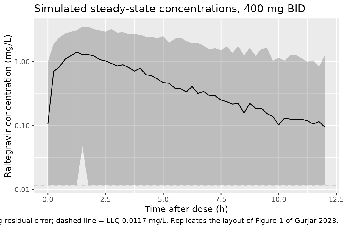
Figure 1 of the paper plots 602 observations between about 0.01 and 17 mg/L. With a 69.9% proportional residual error drawn on the linear scale, the simulated 5th percentile falls below the LLQ (and can be negative) at every time after dose, so the band is drawn from the LLQ upward. The simulated 95th percentile is about 3.5 mg/L near the peak and 0.8 mg/L at 12 h.
PKNCA validation
The paper reports the model-predicted mean (SD; CV%) of AUC0-12, Cmax and C12, and the median Tmax, over its 349 patients (Results, “Population pharmacokinetic modelling”). The simulation is compared with those values using PKNCA on the final steady-state dosing interval.
sim_nca <- sim |>
  dplyr::filter(!is.na(Cc)) |>
  dplyr::select(id, time, Cc, treatment)

dose_df <- events |>
  dplyr::filter(evid == 1) |>
  dplyr::select(id, time, amt, treatment)

conc_obj <- PKNCA::PKNCAconc(sim_nca, Cc ~ time | treatment + id)
dose_obj <- PKNCA::PKNCAdose(dose_df, amt ~ time | treatment + id)

intervals <- data.frame(
  start = t_last_dose,
  end = t_last_dose + 12,
  cmax = TRUE,
  tmax = TRUE,
  auclast = TRUE,
  clast.obs = TRUE
)

nca_res <- PKNCA::pk.nca(PKNCA::PKNCAdata(conc_obj, dose_obj, intervals = intervals))
nca_ind <- as.data.frame(nca_res) |>
  dplyr::select(id, treatment, PPTESTCD, PPORRES) |>
  tidyr::pivot_wider(names_from = PPTESTCD, values_from = PPORRES)
The paper’s half-life is the terminal (beta) half-life computed in
$PK from each patient’s CL, V2, Q and V3. It is computed
here the same way, because PKNCA cannot estimate a terminal slope inside
one 12-h interval.
hl_ind <- sim |>
  dplyr::distinct(id, cl, vc, q, vp) |>
  dplyr::mutate(
    k10 = cl / vc,
    k12 = q / vc,
    k21 = q / vp,
    s = k10 + k12 + k21,
    beta = 0.5 * (s - sqrt(s^2 - 4 * k21 * k10)),
    half.life = log(2) / beta
  ) |>
  dplyr::select(id, half.life)

nca_ind <- dplyr::left_join(nca_ind, hl_ind, by = "id")
Comparison against published values
The paper reports means for every parameter except Tmax, which it reports as a median. The simulated summary therefore uses the same statistics.
sim_summary <- nca_ind |>
  dplyr::group_by(treatment) |>
  dplyr::summarise(
    auclast = mean(auclast),
    cmax = mean(cmax),
    clast.obs = mean(clast.obs),
    half.life = mean(half.life),
    tmax = median(tmax),
    .groups = "drop"
  )

published <- tibble::tribble(
  ~treatment, ~auclast, ~cmax, ~clast.obs, ~half.life, ~tmax,
  "400 mg BID", 8.70, 1.44, 0.29, 9.13, 1.50
)

cmp <- nlmixr2lib::ncaComparisonTable(
  simulated = sim_summary,
  reference = published,
  by = "treatment",
  units = c(
    auclast = "mg*h/L", cmax = "mg/L", clast.obs = "mg/L",
    half.life = "h", tmax = "h"
  ),
  tolerance_pct = 20
)
knitr::kable(
  cmp,
  caption = paste(
    "Simulated (n = 200) vs. published model-predicted values at steady state.",
    "AUC0-12, Cmax, C12 (Clast) and half-life are means; Tmax is a median.",
    "* differs from reference by >20%."
  )
)| NCA parameter | treatment | Reference | Simulated | % diff |
|---|---|---|---|---|
| Cmax (mg/L) | 400 mg BID | 1.44 | 1.42 | -1.7% |
| Tmax (h) | 400 mg BID | 1.5 | 1.5 | +0.0% |
| Clast (mg/L) | 400 mg BID | 0.29 | 0.259 | -10.8% |
| AUClast (mg*h/L) | 400 mg BID | 8.7 | 8.34 | -4.1% |
| t½ (h) | 400 mg BID | 9.13 | 8.92 | -2.3% |
pct <- function(sim, ref) 100 * (sim / ref - 1)
# At steady state AUC0-12 = F * Dose / CL for each subject; the two sides use
# the same drawn CL, so only trapezoidal error separates them.
auc_closed <- sim |>
  dplyr::distinct(id, cl) |>
  dplyr::mutate(auc_cf = 400 / cl) |>
  dplyr::left_join(nca_ind, by = "id")
auc_err <- abs(pct(auc_closed$auclast, auc_closed$auc_cf))
stopifnot(
  median(auc_err) < 1,
  quantile(auc_err, 0.9) < 2
)

# Cohort means against the paper's model-predicted means. The Monte-Carlo SE of
# the AUC mean with a 64% CV and 200 subjects is about 4.5%; a mis-transcribed
# CL/F, volume, dose or unit moves these by tens of percent.
stopifnot(
  abs(pct(sim_summary$auclast, 8.70)) < 15,
  abs(pct(sim_summary$cmax, 1.44)) < 15,
  abs(pct(sim_summary$half.life, 9.13)) < 15,
  # C12 has a CV above 100%, so its mean is noisier.
  abs(pct(sim_summary$clast.obs, 0.29)) < 30,
  sim_summary$tmax >= 1,
  sim_summary$tmax <= 2
)
The simulated means of AUC0-12, Cmax and half-life fall close to the paper’s values, and the median Tmax lies inside the published range of 1.00-2.00 h. The simulated spreads are narrower than the paper’s (published CVs: AUC0-12 94%, Cmax 47%, C12 205%). The paper summarises empirical-Bayes estimates for 349 real patients. Those carry the skewness of a sparse-data fit, while the packaged model draws CL/F from a lognormal with no variability on the other parameters.
Assumptions and deviations
-
IIV scale. Table 2 reports IIV on CL/F as “62.7%”
with no definition. It is read as a coefficient of variation, so omega^2
= log(1 + 0.627^2) = 0.3316. That matches the convention in the same
group’s other packaged models (
Dickinson_2009_atazanavir,Dickinson_2021_dolutegravir,Schipani_2012_lopinavir). The alternative reading, omega x 100 (omega^2 = 0.393), changes the expected mean AUC0-12 from 8.46 to 8.73 mg*h/L. The sampling noise of the comparison above cannot tell these apart, and the paper reports no confidence interval that could decide it. -
Residual error. “Proportional (%) 69.9” is read as
the standard deviation of the proportional error
ERR(1)inY = F*(1 + ERR(1)), i.e.propSd = 0.699. -
Random effects fixed to zero. The control stream
declares etas on Vc, Q, Vp and ka with
$OMEGA 0 FIX. Those etas are omitted from the packaged model because a zero variance has no effect. -
Priors. The
$PRIOR NWPRIprior means (Q 8.5 L/h, V3 113 L, ka 0.21 1/h, V2 223 L) and prior variances (4.6, 46.3, 0.033, 117) only shaped the estimation. The packaged model uses the posterior final estimates from Table 2. Note that the estimated ka (1.12 1/h) moved well away from its prior (0.21 1/h). -
Bioavailability. All parameters are apparent
(divided by F), so
f(depot)is left at 1. -
Screened covariates. Weight, age, sex, ethnicity,
UGT1A1 activity group and the SLC22A6 rs4149170 and rs11568626 genotypes
were screened on CL/F and rejected (Supplementary Table S1). They are
recorded under
covariatesDataExcluded. The non-significant 21% lower CL/F in UGT1A1 low activity (28/28) patients is not in the model. - Dosing. Steady state is approximated by 20 consecutive 400 mg doses every 12 h. Darunavir/ritonavir co-administration is implicit in the parameter values (all patients received it) and is not a covariate.
- No correction notice was found for the article (Europe PMC search, 2026-10-09).