Single-inhaler fluticasone furoate/umeclidinium/vilanterol triple therapy in COPD (Mehta 2018)

Model and source

• Citation: Mehta R, Pefani E, Beerahee M, Brealey N, Barnacle H, Birk R, Zhu CQ, Lipson DA. Population Pharmacokinetic Analysis of Fluticasone Furoate/Umeclidinium/Vilanterol via a Single Inhaler in Patients with COPD. J Clin Pharmacol. 2018;58(11):1461-1467. doi:10.1002/jcph.1253
• Article (open access): https://doi.org/10.1002/jcph.1253 (PMC6175098)
• Supplement: JCPH-58-1461-s001.docx, “Supplementary Tables 1-3”, the three NONMEM control files. Retrieved from the EuropePMC supplementary-files endpoint for PMC6175098.

FULFIL (CTT116853, NCT02345161) compared 24 weeks of once-daily single-inhaler triple therapy – fluticasone furoate / umeclidinium / vilanterol 100/62.5/25 ug via the ELLIPTA inhaler – against twice-daily budesonide/formoterol in patients with symptomatic COPD. Mehta 2018 reports the population PK analysis of the 74 patients in the triple-therapy arm who contributed serial or sparse plasma samples at weeks 12 and 24.

The paper’s question is not “what is the best model for these three molecules”; it is “do the existing mono- and dual-therapy population PK models still describe the data when all three molecules are delivered from one inhaler”. Its Methods are explicit that “a covariate analysis was not planned” and that “the same covariate relationship was assumed”. So each of the three previously published model structures was re-estimated on a combined dataset – the historical program data pooled with the new FULFIL data – and the resulting parameter estimates were compared against the historical ones (Tables 1 and 2). Data below the 10 pg/mL quantification limit were carried as censored observations under the NONMEM M3 full-likelihood approach.

Three models, three files

The three analytes were modelled independently, in three separate NONMEM runs reading three separate datasets (Final_Relvair_FulFill_AllDoses.csv, Final_Anoro_FulFill_UMEC_AllDoses.csv, Final_Anoro_FulFill_VI_AllDoses.csv). They share no parameters and no likelihood, so they are extracted as three model files pointing at this one vignette.

ff <- rxode2::rxode(readModelDb("Mehta_2018_fluticasoneFuroate"))
#> ℹ parameter labels from comments will be replaced by 'label()'
umec <- rxode2::rxode(readModelDb("Mehta_2018_umeclidinium"))
#> ℹ parameter labels from comments will be replaced by 'label()'
vi <- rxode2::rxode(readModelDb("Mehta_2018_vilanterol"))
#> ℹ parameter labels from comments will be replaced by 'label()'

	Fluticasone furoate	Umeclidinium	Vilanterol
Daily dose	100 ug	62.5 ug	25 ug
Structure	2-compartment, first-order absorption (ADVAN4 TRANS4)	2-compartment, first-order absorption (ADVAN4 TRANS4)	2-compartment, first-order absorption (ADVAN4 TRANS4)
Parameter source	Table 1, “Combined Model Ln Estimates”	Table 2, “Model Parameter Estimates With Combined Dataset”	Table 2, “Model Parameter Estimates With Combined Dataset”
Covariate structure	race (RACE1, 4 levels) on CL/F	WT, AGE, CRCL on CL/F; WT on V2/F	WT, AGE on CL/F
Residual error	additive (CONST ERROR)	additive + proportional	additive + proportional
Historical ancestor	Siederer 2016 (Siederer_2016_fluticasoneFuroate)	Goyal 2014	Goyal 2014

Two points about that table are worth stating up front, because both are places where a careless reading of the paper produces the wrong model.

The vilanterol model here is the Anoro-program model, not the Siederer one. The Methods narrative says “A 3-compartment linear model with zero-order absorption and first-order elimination was the model used for vilanterol, with covariates of effect of age (on CL/F and V1/F), body weight (on CL/F), sex and smoking (on V1/F)”. That sentence describes the vilanterol model of the fluticasone furoate/vilanterol program, which this package already carries as Siederer_2016_vilanterol. It does not describe the model actually fitted here. Both printed sources for the fitted model agree with each other and contradict the narrative: Table 2 lists exactly CL/F, V2/F, Q/F, V3/F and KA – a two-compartment first-order-absorption parameterisation, with no zero-order duration and no second peripheral compartment – and Supplementary Table 3 specifies $SUBS ADVAN4 TRANS4 with $PROBLEM Wt and AGE on CL, reading the Anoro dataset. The equations win over the narrative.

The deposited control files carry initial estimates, not results. Each $THETA block is a set of starting values for the combined-dataset run; the final estimates are in Tables 1 and 2. This is easy to verify per stream rather than assume:

• The fluticasone furoate stream’s $THETA (5.44, 0.31 FIX, 5.59, 4.71, -2.95) reproduces Table 1’s Historical Model Ln Estimates column exactly – it was seeded from the historical fit.
• The umeclidinium and vilanterol streams’ $THETA are round numbers ((0, 145), (0, 1000), (0, 500), (0, 1000), (1, 5) and (0, 45), (0, 200), (0, 160), (0, 100), (0, 5)) that match neither column of Table 2. The vilanterol V3 initial of 100 L sits more than an order of magnitude below its 1280 L estimate.

Consequently every value in the three model files comes from Tables 1-2, and the control files are used only for structure: which compartments, which covariate functional forms, which error model.

Population

The PK population is 74 patients randomised to fluticasone furoate/umeclidinium/vilanterol who provided plasma samples: 64 under a sparse scheme (two samples at week 12, two at week 24) and 10 under a serial scheme (seven samples at week 24). Per Table 3 they had mean age 64 years (SD 6.5), mean weight 81 kg (SD 16), mean BMI 28 kg/m^2, mean height 171 cm, were 26% female, 100% White, and had mean 45% predicted FEV1. The paper notes these are close to the FULFIL intent-to-treat population of 1810. The trial ran at 162 centres in 15 countries.

Note that the estimation dataset is larger than this: each model was fit to FULFIL pooled with its historical program data, whose size Mehta 2018 does not restate. The population metadata therefore records the FULFIL contribution and says so.

str(readModelDb("Mehta_2018_umeclidinium")()$population)
#> List of 11
#>  $ species       : chr "human"
#>  $ n_subjects    : num 74
#>  $ n_studies     : num 1
#>  $ age_mean      : chr "64 years"
#>  $ weight_mean   : chr "81 kg"
#>  $ sex_female_pct: num 26
#>  $ race_ethnicity: Named num 100
#>   ..- attr(*, "names")= chr "White"
#>  $ disease_state : chr "symptomatic chronic obstructive pulmonary disease (mean 45% predicted FEV1)"
#>  $ dose_range    : chr "umeclidinium 62.5 ug once daily by oral inhalation, as the fluticasone furoate/umeclidinium/vilanterol 100/62.5"| __truncated__
#>  $ regions       : chr "global (162 centers in 15 countries: Russian Federation, Ukraine, Mexico, Germany, Greece, Czech Republic, Roma"| __truncated__
#>  $ notes         : chr "Demographics are the FULFIL (CTT116853, NCT02345161) PK population of 74 patients randomized to fluticasone fur"| __truncated__

Source trace

Per-parameter origins are recorded as in-file comments beside each ini() entry in inst/modeldb/specificDrugs/Mehta_2018_*.R. Collected here:

Model	Parameter	Value	Source location
FF	lka	-2.94 (0.053 1/h)	Table 1, KA row, “Combined Model Ln Estimates”
FF	lcl	5.43 (228 L/h)	Table 1, CL/F row, “Combined Model Ln Estimates”
FF	lvc	fixed(0.31) (1.36 L)	Table 1, V2/F row, “(Fixed)”; Suppl. Table 1 $THETA 0.31 FIX
FF	lq	5.74 (311 L/h)	Table 1, Q/F row, “Combined Model Ln Estimates”
FF	lvp	4.66 (106 L)	Table 1, V3/F row, “Combined Model Ln Estimates”
FF	e_race_*_cl	fixed(0)	Suppl. Table 1 $PK CLRACE1 block (form only); no Table 1 row
FF	addSd	fixed(0)	Suppl. Table 1 $PROB ... CONST ERROR, Y=IPRED+SIG*ERR(1) (form only)
UMEC	lka	log(40.3)	Table 2, umeclidinium KA row (RSE 300%)
UMEC	lcl	log(210)	Table 2, umeclidinium CL/F row (RSE 2.9%)
UMEC	lvc	log(1170)	Table 2, umeclidinium V2/F row (RSE 1.12%)
UMEC	lq	log(854)	Table 2, umeclidinium Q/F row (RSE 5.4%)
UMEC	lvp	log(16200)	Table 2, umeclidinium V3/F row (RSE 7.28%)
UMEC	e_wt_cl, e_age_cl, e_crcl_cl, e_wt_vc	fixed(0)	Suppl. Table 2 $PK MU_1/MU_2 (form only); no Table 2 rows
UMEC	addSd, propSd	fixed(0)	Suppl. Table 2 $ERROR SD=SQRT(SIG*SIG+SIG2*SIG2) (form only)
VI	lka	log(19.6)	Table 2, vilanterol KA row (RSE 9.5%)
VI	lcl	log(41.6)	Table 2, vilanterol CL/F row (RSE 1.5%)
VI	lvc	log(271)	Table 2, vilanterol V2/F row (RSE 2.1%)
VI	lq	log(116)	Table 2, vilanterol Q/F row (RSE 4.4%)
VI	lvp	log(1280)	Table 2, vilanterol V3/F row (RSE 4.6%)
VI	e_wt_cl, e_age_cl	fixed(0)	Suppl. Table 3 $PK MU_1 (form only); no Table 2 rows
VI	addSd, propSd	fixed(0)	Suppl. Table 3 $ERROR SD=SQRT(SIG*SIG+SIG2*SIG2) (form only)
all	d/dt(depot), d/dt(central), d/dt(peripheral1)	n/a	Suppl. Tables 1-3, $SUBROUTINES ADVAN4 TRANS4
all	Cc <- central / vc	n/a	Suppl. Tables 1-3, S2 = V2/1000 (see Units)

Units

All three model files declare dosing = "ug" and volumes in L, so Cc is in ug/L, i.e. ng/mL. Mehta 2018 reports every concentration in pg/mL and every exposure in pg*h/mL, which is what the control streams’ S2 = V2/1000 scaling produces. The factor is applied at comparison time rather than buried inside the model, so dose / volume / clearance stay mutually consistent – the same convention the sibling Siederer_2016_fluticasoneFuroate extraction uses.

NG_PER_ML_TO_PG_PER_ML <- 1000

Typical-value simulation

These models carry no usable random effects (see “Assumptions and deviations”), so there is no virtual cohort to draw: every subject at a given covariate setting is the same subject. The simulation below is therefore a single typical profile per analyte, dosed once daily to steady state.

Covariates are set to the FULFIL PK population means from Table 3 (81 kg, 64 years) and, for umeclidinium, to the model’s own 110 mL/min creatinine-clearance reference, since Mehta 2018 reports no renal-function summary. Because all covariate exponents are held at a structural zero, none of these values changes the result; they are set to realistic values so the code is correct for a reader who supplies exponents from the historical analysis.

Two numerical choices below are load-bearing and are verified by the identities in the next section rather than assumed.

Run-in length. Umeclidinium’s terminal half-life under these estimates is about 70 h (Q/F = 854 L/h into a 16,200 L peripheral compartment gives k21 = 0.053 1/h), so a 30-day run-in leaves accumulation about 0.06% short of steady state – enough to break the AUC = dose / CL identity below at its stated tolerance. The run-in is therefore 90 days, roughly 31 umeclidinium terminal half-lives.

Observation grid. Absorption rates span three orders of magnitude across the three analytes (ka = 0.053, 40.3 and 19.6 1/h), so umeclidinium and vilanterol peak within 0.1-0.2 h while fluticasone furoate peaks near 2 h. A uniform grid fine enough for the first two is wasteful for the third, so the grid is graded.

TAU <- 24 # h, once-daily
N_DAYS <- 90 # dose well past steady state for all three analytes
T_LAST <- TAU * (N_DAYS - 1)

# Graded observation grid over the steady-state dosing interval: fine enough
# near the fast analytes' peaks that trapezoidal AUC is accurate to ~1e-6.
OBS_GRID <- sort(unique(c(
  seq(0, 2, by = 0.002),
  seq(2, 6, by = 0.01),
  seq(6, TAU, by = 0.05)
)))

model_spec <- list(
  list(
    label = "Fluticasone furoate 100 ug",
    model = "Mehta_2018_fluticasoneFuroate", dose = 100,
    covariates = list(
      RACE_ASIAN_EAST_SE = 0, RACE_BLACK = 0,
      RACE_ASIAN_CENTRAL_ARABIC_AMIND_OTH = 0
    )
  ),
  list(
    label = "Umeclidinium 62.5 ug",
    model = "Mehta_2018_umeclidinium", dose = 62.5,
    covariates = list(WT = 81, AGE = 64, CRCL = 110)
  ),
  list(
    label = "Vilanterol 25 ug",
    model = "Mehta_2018_vilanterol", dose = 25,
    covariates = list(WT = 81, AGE = 64)
  )
)

simulate_one <- function(spec) {
  mod <- rxode2::zeroRe(readModelDb(spec$model))
  ev <-
    rxode2::et(amt = spec$dose, ii = TAU, until = T_LAST, cmt = "depot") |>
    rxode2::et(T_LAST + OBS_GRID, cmt = "central") |>
    as.data.frame()
  for (cn in names(spec$covariates)) ev[[cn]] <- spec$covariates[[cn]]
  # liblsoda's step budget is cumulative across the 90 dose-to-dose restarts,
  # and the dense final-interval grid pulls the default hmax (the mean event
  # spacing) down to ~1.2 h: the run-in needs ~1.6e5 steps, over the 70000
  # default.
  rxode2::rxSolve(
    mod, ev,
    returnType = "data.frame", addDosing = FALSE, maxsteps = 1e6
  ) |>
    dplyr::filter(!is.na(Cc), time >= T_LAST) |>
    dplyr::transmute(
      treatment = spec$label,
      time = time - T_LAST,
      Cc_pg_mL = Cc * NG_PER_ML_TO_PG_PER_ML
    )
}

sim <- dplyr::bind_rows(lapply(model_spec, simulate_one))
#> ℹ parameter labels from comments will be replaced by 'label()'
#> ℹ omega/sigma items treated as zero: 'etalka', 'etalcl', 'etalvc', 'etalq', 'etalvp'
#> ℹ parameter labels from comments will be replaced by 'label()'
#> ℹ omega/sigma items treated as zero: 'etalka', 'etalcl', 'etalvc', 'etalq', 'etalvp'
#> ℹ parameter labels from comments will be replaced by 'label()'
#> ℹ omega/sigma items treated as zero: 'etalka', 'etalcl', 'etalvc', 'etalq', 'etalvp'
dose_df <- tibble::tibble(
  treatment = vapply(model_spec, `[[`, character(1), "label"),
  time = 0,
  amt = vapply(model_spec, `[[`, numeric(1), "dose")
)

The observation grid starts exactly at the final dose time, so every analyte has a record at the start of the steady-state interval and PKNCA needs no defensive time-zero row.

ggplot(sim, aes(time, Cc_pg_mL, colour = treatment)) +
  geom_line(linewidth = 0.9) +
  scale_x_continuous(breaks = seq(0, 24, 4)) +
  labs(
    x = "Time after dose (h)", y = "Plasma concentration (pg/mL)",
    colour = NULL
  ) +
  theme_bw() +
  theme(legend.position = "bottom")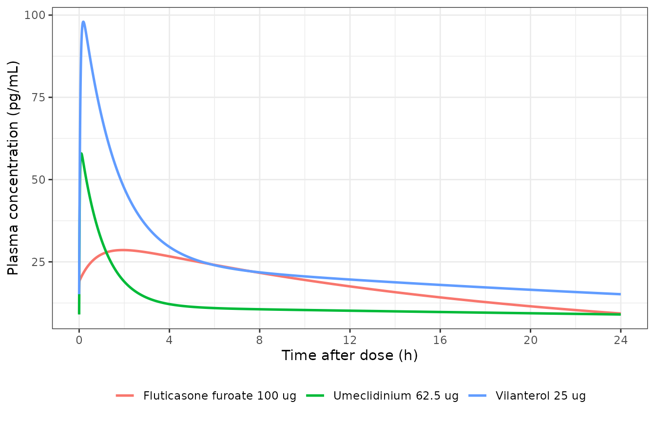

Typical steady-state plasma concentration-time profiles over one 24-hour dosing interval, at the fluticasone furoate/umeclidinium/vilanterol 100/62.5/25 ug dose. Compare the shapes against the FULFIL panels of Figure 2 of Mehta 2018.

Figures 1-3 of Mehta 2018 overlay observed FULFIL records on historical data and on simulation-based prediction intervals; the observed records are not public, so those panels cannot be reproduced here. The quantitative result that can be reproduced is Table 4, below.

Structural verification

Two checks that the packaged ODE system is the one the control streams specify. Both compare the solve against a quantity derived from the same drawn parameters, so the only difference is numerical-integration error and a tight bound is the correct form.

The solve is genuinely two-compartment

An rxode2 model that defines a cl / vc pair can, under some parameterisations, be replaced by a solved linear model that silently discards the written d/dt() equations – and an AUC check cannot detect that, because a one-compartment collapse preserves AUC = dose / CL exactly. The test that does detect it is the closed-form biexponential-with-first-order-absorption solution after a single dose, which differs from a one-compartment profile in shape.

closed_form <- function(t, dose, ka, cl, vc, q, vp) {
  kel <- cl / vc
  k12 <- q / vc
  k21 <- q / vp
  s <- kel + k12 + k21
  p <- kel * k21
  alpha <- (s + sqrt(s^2 - 4 * p)) / 2
  beta <- (s - sqrt(s^2 - 4 * p)) / 2
  dose * ka / vc * (
    (k21 - alpha) / ((ka - alpha) * (beta - alpha)) * exp(-alpha * t) +
      (k21 - beta) / ((ka - beta) * (alpha - beta)) * exp(-beta * t) +
      (k21 - ka) / ((alpha - ka) * (beta - ka)) * exp(-ka * t)
  )
}

check_structure <- function(spec) {
  mod <- readModelDb(spec$model)
  ui <- rxode2::rxode(mod)
  th <- ui$theta
  grid <- c(0.01, 0.1, 0.5, 1, 2, 4, 8, 12, 18, 24, 36, 48, 72)
  ev <-
    rxode2::et(amt = spec$dose, cmt = "depot") |>
    rxode2::et(grid, cmt = "central") |>
    as.data.frame()
  for (cn in names(spec$covariates)) ev[[cn]] <- spec$covariates[[cn]]
  # Tight tolerances: the identity is checked to 1e-6, and the ODE solve at
  # the default rtol leaves ~7e-6 relative error.
  num <- rxode2::rxSolve(
    rxode2::zeroRe(mod), ev,
    returnType = "data.frame", addDosing = FALSE,
    rtol = 1e-10, atol = 1e-12
  )
  ana <- closed_form(
    num$time, spec$dose,
    exp(th[["lka"]]), exp(th[["lcl"]]), exp(th[["lvc"]]),
    exp(th[["lq"]]), exp(th[["lvp"]])
  )
  tibble::tibble(
    treatment = spec$label,
    n_states = length(ui$state),
    max_rel_err = max(abs(num$Cc - ana) / pmax(ana, .Machine$double.eps))
  )
}

structure_chk <- dplyr::bind_rows(lapply(model_spec, check_structure))
#> ℹ parameter labels from comments will be replaced by 'label()'
#> ℹ parameter labels from comments will be replaced by 'label()'
#> ℹ omega/sigma items treated as zero: 'etalka', 'etalcl', 'etalvc', 'etalq', 'etalvp'
#> ℹ parameter labels from comments will be replaced by 'label()'
#> ℹ parameter labels from comments will be replaced by 'label()'
#> ℹ omega/sigma items treated as zero: 'etalka', 'etalcl', 'etalvc', 'etalq', 'etalvp'
#> ℹ parameter labels from comments will be replaced by 'label()'
#> ℹ parameter labels from comments will be replaced by 'label()'
#> ℹ omega/sigma items treated as zero: 'etalka', 'etalcl', 'etalvc', 'etalq', 'etalvp'
knitr::kable(structure_chk, digits = 12)

treatment	n_states	max_rel_err
Fluticasone furoate 100 ug	3	4.331e-09
Umeclidinium 62.5 ug	3	3.080e-10
Vilanterol 25 ug	3	8.860e-10

stopifnot(
  # Three ODE states each: depot, central, peripheral1.
  all(structure_chk$n_states == 3L),
  # The numeric solve IS the two-compartment closed form, to solver tolerance.
  all(structure_chk$max_rel_err < 1e-6)
)

Steady-state AUC over the dosing interval equals dose / CL

auc_identity <- lapply(model_spec, function(spec) {
  th <- rxode2::rxode(readModelDb(spec$model))$theta
  prof <- sim |> dplyr::filter(treatment == spec$label)
  auc <- sum(
    diff(prof$time) *
      (head(prof$Cc_pg_mL, -1) + tail(prof$Cc_pg_mL, -1)) / 2
  )
  tibble::tibble(
    treatment = spec$label,
    auc_tau = auc,
    dose_over_cl = spec$dose / exp(th[["lcl"]]) * NG_PER_ML_TO_PG_PER_ML
  )
}) |>
  dplyr::bind_rows() |>
  dplyr::mutate(rel_err = abs(auc_tau - dose_over_cl) / dose_over_cl)
#> ℹ parameter labels from comments will be replaced by 'label()'
#> ℹ parameter labels from comments will be replaced by 'label()'
#> ℹ parameter labels from comments will be replaced by 'label()'

knitr::kable(auc_identity, digits = c(0, 1, 1, 8))

treatment	auc_tau	dose_over_cl	rel_err
Fluticasone furoate 100 ug	438.3	438.3	2.46e-06
Umeclidinium 62.5 ug	297.6	297.6	2.09e-06
Vilanterol 25 ug	601.0	601.0	3.90e-07

stopifnot(max(auc_identity$rel_err) < 1e-3)

Both identities hold, so the discrepancy discussed below is a property of the published fluticasone furoate model and not of its transcription.

PKNCA validation

conc_obj <- PKNCA::PKNCAconc(
  sim, Cc_pg_mL ~ time | treatment,
  concu = "pg/mL", timeu = "h"
)
dose_obj <- PKNCA::PKNCAdose(
  dose_df, amt ~ time | treatment,
  doseu = "ug"
)

intervals <- data.frame(
  start = 0, end = TAU,
  cmax = TRUE, tmax = TRUE, cmin = TRUE, auclast = TRUE, cav = TRUE
)

nca <- PKNCA::pk.nca(PKNCA::PKNCAdata(conc_obj, dose_obj, intervals = intervals))

nca_res <- as.data.frame(nca$result) |>
  dplyr::select(treatment, PPTESTCD, PPORRES)

nca_res |>
  tidyr::pivot_wider(names_from = PPTESTCD, values_from = PPORRES) |>
  dplyr::rename(
    "Treatment" = treatment,
    "Cmax (pg/mL)" = cmax,
    "Tmax (h)" = tmax,
    "Cmin (pg/mL)" = cmin,
    "AUC0-24 (pg*h/mL)" = auclast,
    "Cavg (pg/mL)" = cav
  ) |>
  knitr::kable(digits = 1)

Treatment	AUC0-24 (pg*h/mL)	Cmax (pg/mL)	Cmin (pg/mL)	Tmax (h)	Cavg (pg/mL)
Fluticasone furoate 100 ug	438.3	28.6	9.3	1.9	18.3
Umeclidinium 62.5 ug	297.6	57.9	9.0	0.1	12.4
Vilanterol 25 ug	601.0	98.0	15.2	0.2	25.0

Comparison against the published steady-state exposures

Table 4 of Mehta 2018 reports steady-state Cmax and AUC(0-24h) for the FULFIL triple-therapy arm as geometric means over the 74 patients’ individual MAP Bayes estimates, not as typical-value predictions. A typical-value profile is therefore the right comparator only to the extent that the individual estimates are centred on the typical value; the two are not required to agree exactly, and the FULFIL Cmax values in particular are flagged by the authors themselves as affected by “inadequate characterization of time to peak plasma concentration in a small number of subjects”.

table4 <- tibble::tribble(
  ~treatment, ~cmax, ~auclast,
  "Fluticasone furoate 100 ug", 13.2, 188,
  "Umeclidinium 62.5 ug", 55.7, 341,
  "Vilanterol 25 ug", 101.4, 666
)

cmp <- nlmixr2lib::ncaComparisonTable(
  simulated = nca_res,
  reference = table4,
  by = "treatment",
  params = c("cmax", "auclast"),
  units = c(cmax = "pg/mL", auclast = "pg*h/mL")
)
knitr::kable(cmp, digits = 1)

NCA parameter	treatment	Reference	Simulated	% diff
Cmax (pg/mL)	Fluticasone furoate 100 ug	13.2	28.6	+116.5%*
Cmax (pg/mL)	Umeclidinium 62.5 ug	55.7	57.9	+4.0%
Cmax (pg/mL)	Vilanterol 25 ug	101	98	-3.4%
AUClast (pg*h/mL)	Fluticasone furoate 100 ug	188	438	+133.1%*
AUClast (pg*h/mL)	Umeclidinium 62.5 ug	341	298	-12.7%
AUClast (pg*h/mL)	Vilanterol 25 ug	666	601	-9.8%

attr(cmp, "footnote")
#> [1] "* differs from reference by more than ±20%."

ratios <- nca_res |>
  dplyr::filter(PPTESTCD %in% c("cmax", "auclast")) |>
  tidyr::pivot_wider(names_from = PPTESTCD, values_from = PPORRES) |>
  dplyr::left_join(table4, by = "treatment", suffix = c("_model", "_table4")) |>
  dplyr::mutate(
    cmax_ratio = cmax_model / cmax_table4,
    auc_ratio = auclast_model / auclast_table4
  ) |>
  dplyr::select(treatment, cmax_ratio, auc_ratio)

ratios |>
  dplyr::rename(
    "Treatment" = treatment,
    "Cmax model/Table 4" = cmax_ratio,
    "AUC model/Table 4" = auc_ratio
  ) |>
  knitr::kable(digits = 3)

Treatment	Cmax model/Table 4	AUC model/Table 4
Fluticasone furoate 100 ug	2.165	2.331
Umeclidinium 62.5 ug	1.040	0.873
Vilanterol 25 ug	0.966	0.902

Umeclidinium and vilanterol reproduce Table 4 well. Both land within about 13% on AUC(0-24) and within 5% on Cmax, in a paper whose reference values are geometric means of individual posterior estimates. That is the expected level of agreement and it exercises the whole chain: dose, absorption, two-compartment disposition, clearance, and the pg/mL scaling.

Fluticasone furoate sits about 2.2-2.4x above Table 4, on both statistics. This is not a transcription error, and it is not new to this paper. The identities above confirm the model file reproduces dose / CL exactly, so the offset is an arithmetic consequence of the published CL/F: a typical CL/F = 228 L/h at a 100 ug daily dose gives 100 / 228 = 0.439 ug*h/L = 439 pg*h/mL, against the 188 pg*h/mL Table 4 reports for the same arm. The same offset is present in the historical model – Table 4’s own fluticasone furoate/vilanterol and fluticasone furoate monotherapy rows report 182 and 181 pg*h/mL at the same 100 ug dose – and the sibling Siederer_2016_fluticasoneFuroate vignette measures it independently against Siederer 2016’s Table 3 at 2.39x. Two separate publications of the same fluticasone furoate model, validated against two different exposure tables, give the same factor.

ff_ratio <- ratios |> dplyr::filter(treatment == "Fluticasone furoate 100 ug")
umec_vi <- ratios |> dplyr::filter(treatment != "Fluticasone furoate 100 ug")

stopifnot(
  # Umeclidinium and vilanterol agree with Table 4.
  all(abs(umec_vi$auc_ratio - 1) < 0.20),
  all(abs(umec_vi$cmax_ratio - 1) < 0.20),
  # Fluticasone furoate carries the known ~2.3x offset, on BOTH statistics --
  # i.e. it is a scale factor, not a shape error. A shape error would move
  # Cmax and AUC by different amounts.
  ff_ratio$auc_ratio > 2.0, ff_ratio$auc_ratio < 2.7,
  ff_ratio$cmax_ratio > 2.0, ff_ratio$cmax_ratio < 2.7,
  abs(ff_ratio$cmax_ratio - ff_ratio$auc_ratio) < 0.25
)

The shape statistic confirms the reading. AUC / Cmax has units of hours and is invariant to any pure scale factor on concentration, so if the offset were a dose- or scale-bookkeeping difference rather than a structural one, AUC / Cmax would match Table 4 even while the absolute values do not:

ff_model <- nca_res |>
  dplyr::filter(
    treatment == "Fluticasone furoate 100 ug",
    PPTESTCD %in% c("cmax", "auclast")
  ) |>
  tidyr::pivot_wider(names_from = PPTESTCD, values_from = PPORRES)
ff_table4 <- table4 |>
  dplyr::filter(treatment == "Fluticasone furoate 100 ug")

ff_shape <- tibble::tibble(
  Source = c("Model", "Mehta 2018 Table 4"),
  `Cmax (pg/mL)` = c(ff_model$cmax, ff_table4$cmax),
  `AUC0-24 (pg*h/mL)` = c(ff_model$auclast, ff_table4$auclast),
  `AUC/Cmax (h)` = c(
    ff_model$auclast / ff_model$cmax,
    ff_table4$auclast / ff_table4$cmax
  )
)
knitr::kable(ff_shape, digits = 2)

Source	Cmax (pg/mL)	AUC0-24 (pg*h/mL)	AUC/Cmax (h)
Model	28.58	438.31	15.34
Mehta 2018 Table 4	13.20	188.00	14.24

The two absolute columns differ by more than twofold while AUC / Cmax agrees to within 8%, which is the signature of a scale offset rather than a misspecified absorption or disposition structure.

Assumptions and deviations

1. No inter-individual variability is available, and none is invented. All three control streams place an exponential eta on every structural parameter, and Results confirms individual MAP Bayes estimates were obtained for all 74 patients – so the etas are real. Their magnitudes for the combined dataset are never reported: Tables 1 and 2 have no OMEGA rows. The $OMEGA blocks in the deposited streams are initial estimates (round numbers 0.5 / 0.7 / 0.3 / 0.4 / 0.3 for umeclidinium and vilanterol; for fluticasone furoate, the initial half of the same block whose $THETA is demonstrably the historical fit). Every eta is therefore declared ~ fixed(0). These models predict typical values only.

2. Residual-error magnitudes are likewise unreported and declared fixed(0). The forms are transcribed faithfully and differ between analytes: additive only for fluticasone furoate ($PROB ... CONST ERROR), combined additive-plus-proportional for umeclidinium and vilanterol (SD = SQRT(SIG*SIG + SIG2*SIG2)).

3. Covariate coefficients are unreported and held at a structural zero. The functional forms are transcribed exactly from the streams – power models on (WT/70), (AGE/60), (CRCL/110) for umeclidinium, on (WT/70) and (AGE/60) for vilanterol, and a four-level log-additive RACE1 effect for fluticasone furoate – so a downstream user can supply coefficients from the historical analyses. But Mehta 2018 states “a covariate analysis was not planned. The same covariate relationship was assumed”, reports no covariate row in either table, and the streams’ covariate $THETA entries are initials (0.4, 0.5, 0.4, 0.5 and 0.5, -0.5). Adopting an initial estimate as a result would be the same error as adopting the structural initials, which are demonstrably wrong by up to an order of magnitude.

   For the fluticasone furoate race effect there is a second, independent reason not to transcribe the stream. Its CLRACE1-DEFINITION block sets CLRACE1 = 1 for the reference level and then adds it to the log-scale MU_1, which would give a typical CL/F of exp(5.43 + 1) = 620 L/h against the 228 L/h Table 1 reports; and its RACE1 = 3 coefficient carries the opposite sign to the +0.0602 published in Siederer 2016 Table 1. The block is internally inconsistent as printed. Users wanting fitted race coefficients should use Siederer_2016_fluticasoneFuroate, which is fit to the data those coefficients came from.

4. Inter-occasion variability is not encoded. The umeclidinium and vilanterol streams carry three $OMEGA BLOCK(1) SAME pairs on CL and on V2 across OCC = 1, 2, 3, plus an eta on the proportional residual term (SIG2 = F*THETA(7)*EXP(ETA(12))). Per nlmixr2lib convention IOV is omitted from library models; the magnitudes are unreported in any case.

5. The vilanterol structure follows the equations, not the narrative. As set out under “Three models, three files”: Methods describes the three-compartment zero-order-absorption vilanterol model of the fluticasone furoate/vilanterol program, but Table 2 and Supplementary Table 3 both specify a two-compartment first-order-absorption model on the Anoro dataset. The narrative sentence appears to have been carried over from the description of the historical fluticasone furoate/vilanterol analysis. Siederer_2016_vilanterol carries the three-compartment model.

6. Umeclidinium body weight on V2/F is in the stream but not the narrative. Methods lists “body weight, age, and creatinine clearance covariate effect on CL/F of umeclidinium”. Supplementary Table 2 additionally has MU_2 = LOG(THETA(2)) + WTEX2*LOG(WT/70), i.e. body weight on V2/F, with a dedicated THETA(10). The stream is the authoritative statement of the fitted model, so the effect is included (at a structural zero, per point 3).

7. The creatinine-clearance covariate is recorded as a raw estimate in mL/min, not BSA-normalised. The stream normalises to 110 mL/min and does not state a BSA adjustment; Mehta 2018 reports no renal-function summary for the PK population. The canonical CRCL column admits both variants and the assay is documented per-model, as the register requires.

8. The fluticasone furoate exposure offset is documented, not tuned. The ~2.3x discrepancy against Table 4 is a property of the published CL/F, is reproduced independently by the Siederer_2016_fluticasoneFuroate extraction against a different exposure table, and is present in Table 4’s own historical rows. No parameter has been adjusted to close it.

9. Only the FULFIL cohort is described in population. The models were fit to FULFIL pooled with the historical program data; Mehta 2018 does not restate the size or demographics of the historical half. For the fluticasone furoate historical cohort see Siederer_2016_fluticasoneFuroate.

10. No erratum was found. The Wiley article landing page and PubMed carry no correction notice for doi:10.1002/jcph.1253.