DOTATATE whole-body PBPK for peptide receptor radionuclide therapy (Budiansah 2025)
Source:vignettes/articles/Budiansah_2025_dotatate_pbpk.Rmd
Budiansah_2025_dotatate_pbpk.Rmd
library(nlmixr2lib)
library(rxode2)
library(PKNCA)
library(dplyr)
library(tidyr)
library(ggplot2)
library(knitr)
The model
Budiansah et al. (EJNMMI Physics 2025;12:26, doi:10.1186/s40658-025-00726-7)
asked how much accuracy and precision is lost when the absorbed doses
that guide peptide receptor radionuclide therapy (PRRT) are estimated
from a single post-injection image instead of the full
five-image series. The vehicle for that question is a whole-body
physiologically-based pharmacokinetic (PBPK) model of the
somatostatin-receptor (sst2) targeted peptide DOTATATE, fitted within a
non-linear mixed-effects framework to [111In]In-DOTA-TATE
biokinetics in eight patients.
The single-time-point analysis itself is a study design, not a model. What is extractable, and what this vignette packages, is the PBPK model with the paper’s parameter setting II – the set selected over setting I by an Akaike weight of nearly 100 %.
mod <- rxode2::rxode(nlmixr2lib::readModelDb("Budiansah_2025_dotatate_pbpk"))
length(mod$state)
#> [1] 114
The structural equations and every fixed physiological parameter come from the upstream framework paper (Kletting et al., J Nucl Med 2016;57:503-8, doi:10.2967/jnumed.115.164699) and its supplemental data, which Budiansah 2025 Table S1 reproduces. The ten estimated parameters come from Budiansah 2025 Table 1.
Two circulations, one receptor pool
The paper writes two parallel systems – one for unlabelled and one for labelled peptide – coupled in exactly two places: physical decay converts labelled into unlabelled peptide, and both compete for one conserved pool of sst2 binding sites.
This packaging writes that pair in the algebraically equivalent
total / labelled basis. Summing the paper’s two printed
equations cancels every decay term, so the total-peptide states obey the
same equations with no decay, while the labelled states keep
-lambda_phy and lose their decay-gain term. The paper’s
unlabelled states are recovered as
P_unl = P_tot - P_lab * 0.082 nmol. The change of basis
removes a scale separation of about 1e3: 140 MBq of 111In
is only 0.082 nmol of the 75 nmol of DOTATATE injected. It also lets the
labelled system be dosed with 1, so every labelled state reads directly
as a fraction of the injected activity. The structural checks below verify the basis
change against the identity it implies.
Regions
Ten sst2-positive regions (tumour, liver, spleen, kidneys, GI plus pancreas, muscle, red marrow, prostate or uterus, adrenals and a lumped rest of body) each carry vascular, interstitial, receptor-bound and internalised sub-compartments. The kidneys add a fifth intracellular pool fed by glomerular filtration. Five sst2-negative regions (lungs, skin, adipose, heart, bone) carry vascular and interstitial pools, and the brain is vascular-only because its permeability-surface product is set to zero. Arteries, veins and an irreversibly serum-protein-bound pool complete the structure. Spleen and GI drain into the liver through the portal circulation (Figure 1 of the paper); everything else drains straight to the veins.
Population
The cohort is eight patients – four with metastasised neuroendocrine
tumours (NET) and four with meningiomas – all scheduled for two to three
cycles of [90Y]Y-DOTA-TATE PRRT. Each received 75 +/- 10
nmol of DOTATATE labelled with 140 +/- 14 MBq of 111In as a 51 +/- 8 min
intravenous infusion, with arginine and lysine co-infused for renal
protection. Serum was counted at 5 and 15 min, 0.5, 1, 2 and 4 h and 1,
2 and 3 d; planar whole-body scintigraphy was performed at 2, 4, 24, 48
and 72 h.
mod$meta$population[c("species", "n_subjects", "disease_state", "dose_range")] |>
  unlist() |>
  as.data.frame() |>
  setNames("value") |>
kable()| value | |
|---|---|
| species | human |
| n_subjects | 8 |
| disease_state | Four patients with metastasised neuroendocrine tumours and four with meningiomas, all scheduled for two to three cycles of [90Y]Y-DOTA-TATE peptide receptor radionuclide therapy. |
| dose_range | 75 +/- 10 nmol DOTATATE labelled with 140 +/- 14 MBq 111In, given as a 51 +/- 8 min intravenous infusion |
The per-patient covariates
Budiansah 2025 tabulates no patient characteristics; its eight patients are a subset of the nine-patient cohort of the upstream Kletting 2016 framework paper, whose Table 1 is the only available source of the body surface areas, measured 51Cr-EDTA glomerular filtration rates, organ volumes, tumour volumes, sexes and disease types.
The mapping onto Budiansah’s patient numbering is fixed by two independent checks in the paper itself. Budiansah Figure S2 states that patient 5 had a splenectomy, and Kletting Table 1 marks patient P6 as the splenectomised one; Budiansah Figure 3 gives patient 4 a tumour volume of 2.8 mL, and Kletting P4 has a single 3 mL lesion. With four meningiomas first and four NETs after, that makes Budiansah 1-4 = Kletting P1-P4 and Budiansah 5-8 = Kletting P6-P9, with Kletting P5 (whose tumour volume is a whole-liver surrogate) excluded.
cohort <- data.frame(
  id            = 1:8,
  kletting      = c("P1", "P2", "P3", "P4", "P6", "P7", "P8", "P9"),
  disease       = c(rep("meningioma", 4), rep("NET", 4)),
  TUMTP_NET     = c(0, 0, 0, 0, 1, 1, 1, 1),
  SEXF          = c(0, 0, 1, 0, 1, 0, 1, 0),
  BSA           = c(1.94, 1.99, 1.94, 2.05, 1.81, 1.86, 1.57, 1.81),
  gfr_L_min     = c(0.11, 0.12, 0.090, 0.13, 0.092, 0.059, 0.028, 0.050),
  ORGVOL_SPLEEN = c(198, 178, 110, 243, NA, 146, 128, 161),
  ORGVOL_LIVER  = c(1811, 1824, 1500, 1896, 1897, 1804, 1610, 1900),
  ORGVOL_KIDNEY = c(193, 185, 125, 206, 156, 157, 233, 156),
  tumour_mL     = c(107, 116, 2.5, 3, 34, 134, 15, 18)
)

cohort <- cohort |>
  mutate(
    # Splenectomy: a small positive placeholder keeps the spleen sub-volume
    # divisions finite; that subject's spleen output is dropped below.
    splenectomy   = is.na(ORGVOL_SPLEEN),
    ORGVOL_SPLEEN = ifelse(splenectomy, 1, ORGVOL_SPLEEN),
    # Body weight and hematocrit are "individually measured" per Table S1 but
    # are tabulated in no available source. See Assumptions and deviations.
    WT            = 71,
    HCT           = ifelse(SEXF == 1, 40, 45),
    # The canonical CRCL is BSA-normalised; Kletting Table 1 reports absolute
    # L/min, so normalise on the way in (model() undoes it exactly).
    CRCL          = gfr_L_min * 1000 * 1.73 / BSA,
    TUM_VOL       = tumour_mL * 1000
  )

cohort |>
  select(id, kletting, disease, SEXF, BSA, gfr_L_min, ORGVOL_KIDNEY,
         ORGVOL_LIVER, ORGVOL_SPLEEN, tumour_mL) |>
kable(caption = "Cohort covariates, from Kletting 2016 Table 1.")| id | kletting | disease | SEXF | BSA | gfr_L_min | ORGVOL_KIDNEY | ORGVOL_LIVER | ORGVOL_SPLEEN | tumour_mL |
|---|---|---|---|---|---|---|---|---|---|
| 1 | P1 | meningioma | 0 | 1.94 | 0.110 | 193 | 1811 | 198 | 107.0 |
| 2 | P2 | meningioma | 0 | 1.99 | 0.120 | 185 | 1824 | 178 | 116.0 |
| 3 | P3 | meningioma | 1 | 1.94 | 0.090 | 125 | 1500 | 110 | 2.5 |
| 4 | P4 | meningioma | 0 | 2.05 | 0.130 | 206 | 1896 | 243 | 3.0 |
| 5 | P6 | NET | 1 | 1.81 | 0.092 | 156 | 1897 | 1 | 34.0 |
| 6 | P7 | NET | 0 | 1.86 | 0.059 | 157 | 1804 | 146 | 134.0 |
| 7 | P8 | NET | 1 | 1.57 | 0.028 | 233 | 1610 | 128 | 15.0 |
| 8 | P9 | NET | 0 | 1.81 | 0.050 | 156 | 1900 | 161 | 18.0 |
Source trace
| Quantity | Source |
|---|---|
| Two-circulation structure; equations for internalised, bound, vascular, interstitial, intracellular, arterial, venous and protein-bound peptide | Kletting 2016 supplemental data, equations S1-S13 (reproduced by Budiansah 2025 Fig. 1) |
| Portal drainage: spleen and GI into the liver | Budiansah 2025 Figure 1 (arrows into the liver box) |
| [R_K,0] 4.55, [R_L,0] 0.94, [R_S,0] 7.37, [R_TU,0] 15.9, [R_Rest,0] 0.36 nmol/L | Budiansah 2025 Table 1 (setting II) |
| k_on,Alb 5.50e-4 /min | Budiansah 2025 Table 1 |
| lambda_int,K 2.36e-3, lambda_int,TU 1.39e-3 /min | Budiansah 2025 Table 1 |
| lambda_deg,NT 1.01e-4, lambda_deg,TU 1.15e-4 /min | Budiansah 2025 Table 1 |
| Interindividual variability, 19-101 % CV | Budiansah 2025 Table 1 ‘RE (%RSE)’ column; omega^2 = log(CV^2 + 1) |
| Proportional residual error per region, 5.3-23 % | Budiansah 2025 Table 1, parameter a of equation 2 |
| k_off 0.04 /min, K_D 0.4 nmol/L, lambda_phy 1.71e-4 (111In) and 1.80e-4 (90Y) /min | Budiansah 2025 Table S1 |
| V_P = 2.8 (male) or 2.4 (female) x (1 - H) x BSA; F = 1.23 x V_P | Budiansah 2025 Table S1 |
| Organ volume, vascular, interstitial and flow fractions; alpha ratios; permeability densities | Budiansah 2025 Table S1 |
| sst2 densities of non-delineated organs relative to the kidneys | Budiansah 2025 Table S1 (regional sst2 expression of Boy et al.) |
| Tumour-type switches: interstitial 0.3/0.23, vascular 0.1/0.11, perfusion 1.0/0.9, permeability 0.2/0.31 | Budiansah 2025 Table S1 and Study workflow (setting II prior knowledge) |
| phi 0.66, f_ex 0.98, V_K,intra = (V_K,total - V_K,int - V_K,v) x 2/3 | Budiansah 2025 Table S1 |
| Per-patient BSA, GFR, organ and tumour volumes, sex, disease | Kletting 2016 Table 1 |
| Reference TIACs used as the validation answer key | Budiansah 2025 Table S3 |
| Biokinetic curves reproduced below | Budiansah 2025 Figure S1 |
| Kidney self-absorbed dose factor 2.93e-5 (male) / 3.18e-5 (female) Gy/min/MBq | Budiansah 2025 Methods, ‘Data analysis’ |
Simulation
Both circulations are dosed as the 51 min infusion: 75 nmol of total peptide and 1 unit of labelled activity, so the labelled states read as a fraction of the injected activity. The paper integrates TIACs from time zero to 30 000 min, so the grid runs that far and is dense early where the serum falls fastest.
tgrid <- unique(c(seq(0, 120, by = 2), seq(122, 1440, by = 6),
                  seq(1450, 30000, by = 50)))

# All six endpoints are algebraic observables, so rxode2 maps dvid 1-6 onto the
# six endpoint slots 115-120. An observation row therefore needs both a real ODE
# state in `cmt` and a `dvid`: naming an observable in `cmt` is the
# slot-renumbering antipattern, and a bare state name without `dvid` fails with
# "'dvid'->'cmt' or 'cmt' on observation record". One dvid is enough, because
# every algebraic observable is returned on every solved row.
tag_obs <- function(ev) {
  d <- as.data.frame(ev)
  d$dvid <- ifelse(d$evid == 0, 1L, NA_integer_)
  d$cmt[d$evid == 0] <- "pven_tot"
  d
}

dose_events <- function(ids) {
  tag_obs(
    et(amt = 75, cmt = "pven_tot", dur = 51, id = ids) |>
      et(amt = 1, cmt = "pven_lab", dur = 51, id = ids) |>
      et(tgrid, cmt = "pven_tot", id = ids)
  )
}

modz <- rxode2::zeroRe(mod)   # typical-value (no IIV, no residual error) run

sim <- rxSolve(
  modz,
  events = dose_events(cohort$id),
  iCov   = cohort[, c("id", "TUMTP_NET", "SEXF", "BSA", "HCT", "WT", "CRCL",
                      "ORGVOL_KIDNEY", "ORGVOL_LIVER", "ORGVOL_SPLEEN",
                      "TUM_VOL")],
  atol = 1e-12, rtol = 1e-10, omega = NA, sigma = NA, addDosing = FALSE
) |>
  as.data.frame()

nrow(sim)
#> [1] 6824
length(unique(sim$id))   # rxSolve silently drops subjects on some failures
#> [1] 8
stopifnot(length(unique(sim$id)) == nrow(cohort))
Structural checks
Before comparing anything to the paper, two internal identities confirm that all 114 ODEs are wired consistently. Neither depends on the published parameter values, so they test the implementation rather than the fit.
Mass balance is exact
Total peptide is conserved: whatever is not in a body compartment must be in the cumulative urinary-excretion or degradation bookkeeping states.
The labelled system reduces exactly to the total system
Because labelled and unlabelled peptide are assumed kinetically
identical, the labelled states must satisfy, for every compartment
i,
with D the total peptide dose. This is an exact
consequence of the printed equations, and it constrains all 57
compartments at once – perfusion, permeability, binding,
internalisation, degradation, filtration and the portal loop all have to
be identical between the two systems for it to hold.
The identity is exact only for an instantaneous input, because the labelled input during a finite infusion is not itself decay-weighted. So the residual should be a few tenths of a percent for the 51 min infusion, should fall roughly in proportion to the infusion duration, and should vanish into solver noise for a bolus.
lambda_phy <- 1.71e-4

id_err <- function(dur) {
  ev <- if (is.na(dur)) {
    et(amt = 75, cmt = "pven_tot", id = 1L) |>
      et(amt = 1, cmt = "pven_lab", id = 1L)
  } else {
    et(amt = 75, cmt = "pven_tot", dur = dur, id = 1L) |>
      et(amt = 1, cmt = "pven_lab", dur = dur, id = 1L)
  }
  ev <- tag_obs(et(ev, tgrid, cmt = "pven_tot", id = 1L))
  s <- rxSolve(modz, events = ev,
               iCov = cohort[1, c("id", "TUMTP_NET", "SEXF", "BSA", "HCT", "WT",
                                  "CRCL", "ORGVOL_KIDNEY", "ORGVOL_LIVER",
                                  "ORGVOL_SPLEEN", "TUM_VOL")],
               atol = 1e-12, rtol = 1e-10, omega = NA, sigma = NA,
               addDosing = FALSE) |>
    as.data.frame()
  s <- s[s$time > ifelse(is.na(dur), 5, dur + 5), ]
  probe <- c("pv_liver", "pint_kidney", "rp_tumor", "pintern_kidney",
             "pintra_kidney", "pprp", "pven", "part")
  max(vapply(probe, function(st) {
    pred <- s[[paste0(st, "_tot")]] / 75 * exp(-lambda_phy * s$time)
    # Score the identity over each compartment's top six orders of magnitude,
    # where the solve is numerically resolved. In the deep tail several states
    # decay to ~1e-30, far below the 1e-12 absolute tolerance, so a relative
    # error taken there measures solver noise rather than the model.
    keep <- pred > 1e-6 * max(pred)
    max(abs(s[[paste0(st, "_lab")]][keep] - pred[keep]) / pred[keep])
  }, numeric(1)))
}

identity_check <- data.frame(
  infusion_min   = c(51, 10, 1, NA),
  max_rel_error  = vapply(c(51, 10, 1, NA), id_err, numeric(1))
)
identity_check |>
  mutate(infusion_min = ifelse(is.na(infusion_min), "bolus",
                               as.character(infusion_min))) |>
  rename("Infusion (min)" = infusion_min,
         "Max relative error over 8 compartments" = max_rel_error) |>
kable(digits = 10)| Infusion (min) | Max relative error over 8 compartments |
|---|---|
| 51 | 0.0048704016 |
| 10 | 0.0009323257 |
| 1 | 0.0000868400 |
| bolus | 0.0000003134 |
The residual falls by roughly an order of magnitude for each order of magnitude of infusion duration, and for a bolus reaches 3e-7 – four orders of magnitude below the 51 min value – which is exactly the predicted behaviour. All 114 states are consistent.
The 51 min figure is a genuine structural residual: it is unchanged to three significant figures whether the identity is scored over each compartment’s top four, six, eight or ten orders of magnitude, because the finite-infusion approximation biases the well-resolved early profile where the peptide actually is. The bolus figure behaves in the opposite way – it shrinks monotonically as the scoring window is tightened (1.7e-5, 3.2e-6, 3.1e-7, 1.0e-8 at cut-offs of 1e-10, 1e-8, 1e-6 and 1e-4 of each compartment’s peak) – which is the signature of accumulated solver noise in the decayed tail rather than of a broken equation.
Reproducing the published reference TIACs
Table S3 of the paper reports, per patient, the reference time-integrated activity coefficients (rTIACs) from the all-time-point fit – the quantity the whole dosimetry analysis rests on. Those are individual values from a fitted mixed-effects model; the simulation here uses typical values with every eta set to zero, so the comparison probes whether the published fixed effects put each region at the right level, not whether individual predictions are recovered.
trap <- function(time, y) sum(diff(time) * (head(y, -1) + tail(y, -1)) / 2)

pred_tiac <- sim |>
  group_by(id) |>
  summarise(across(c(Aserum, Abody, Akidney, Aspleen, Aliver, Atumor),
                   ~ trap(time, .x)), .groups = "drop")

obs_tiac <- data.frame(
  id      = 1:8,
  Aserum  = c(20, 19, 24, 18, 28, 28, 62, 44),
  Abody   = c(956, 904, 997, 1099, 1151, 1093, 1641, 2237),
  Akidney = c(139, 114, 106, 188, 144, 82, 144, 211),
  Aspleen = c(100, 81, 121, 164, NA, 54, 83, 226),
  Aliver  = c(161, 108, 97, 108, 194, 198, 157, 331),
  Atumor  = c(52, 168, 0.90, 4.7, 49, 98, 23, 7.8)
)

# Patient 5 is splenectomised and contributed no spleen data.
pred_tiac$Aspleen[cohort$splenectomy] <- NA

long <- bind_rows(
  pred_tiac |> pivot_longer(-id, names_to = "region", values_to = "predicted"),
  obs_tiac  |> pivot_longer(-id, names_to = "region", values_to = "published") |>
    select(id, region, published)
) |>
  group_by(id, region) |>
  summarise(predicted = first(na.omit(predicted)),
            published = first(na.omit(published)), .groups = "drop") |>
  mutate(ratio = predicted / published)

long |>
  select(id, region, ratio) |>
  pivot_wider(names_from = region, values_from = ratio) |>
  select(id, Aserum, Abody, Akidney, Aspleen, Aliver, Atumor) |>
  rename("Patient" = id, "Serum" = Aserum, "Whole body" = Abody,
         "Kidneys" = Akidney, "Spleen" = Aspleen, "Liver" = Aliver,
         "Tumour" = Atumor) |>
  kable(digits = 2,
caption = "Predicted / published rTIAC ratio, typical values.")| Patient | Serum | Whole body | Kidneys | Spleen | Liver | Tumour |
|---|---|---|---|---|---|---|
| 1 | 1.06 | 0.95 | 0.44 | 1.03 | 0.79 | 1.44 |
| 2 | 1.04 | 0.95 | 0.49 | 1.10 | 1.13 | 0.46 |
| 3 | 1.08 | 0.86 | 0.42 | 0.53 | 1.22 | 2.18 |
| 4 | 1.04 | 0.72 | 0.31 | 0.70 | 1.12 | 0.41 |
| 5 | 0.93 | 0.70 | 0.38 | NA | 0.75 | 0.53 |
| 6 | 1.21 | 1.18 | 0.89 | 2.04 | 0.93 | 1.36 |
| 7 | 1.01 | 1.03 | 1.07 | 1.66 | 1.51 | 0.92 |
| 8 | 0.90 | 0.59 | 0.38 | 0.59 | 0.64 | 2.52 |
long |>
  group_by(region) |>
  summarise(`median ratio` = median(ratio, na.rm = TRUE), .groups = "drop") |>
  rename("Region" = region) |>
kable(digits = 2, caption = "Median across the eight patients.")| Region | median ratio |
|---|---|
| Abody | 0.90 |
| Akidney | 0.43 |
| Aliver | 1.02 |
| Aserum | 1.04 |
| Aspleen | 1.03 |
| Atumor | 1.14 |
Five of the six regions land close to the published individual values: serum 1.04, whole body 0.90, spleen 1.03, liver 1.02 and tumour 1.14. For a typical-value simulation compared against individual empirical-Bayes fits from a model whose interindividual variability runs from 19 % to 101 % CV, that is about as close as this comparison can get.
The kidney is the exception, and it is off by a
consistent factor of roughly 2.3 rather than scattering. That is a
property of the published numbers, not of the implementation, and the
model makes the reason falsifiable. In this model the kidneys and the
spleen are structurally near-identical – same internalisation rate
(Table S1 sets lambda_int,S = lambda_int,K), same
degradation rate
(lambda_deg,S = lambda_deg,NT = lambda_deg,K), and
retention dominated by the internalised pool in both. They differ
essentially only in receptor number. So equalising the receptor number
should equalise the TIACs:
r0 <- cohort |>
  transmute(id,
            r0_kidney = 4.55 * ORGVOL_KIDNEY / 1000,
            r0_spleen = 7.37 * ORGVOL_SPLEEN / 1000)

equalised <- rxode2::ini(modz, lrdens_kidney = log(7.37 * 198 / 193))
#> ℹ change initial estimate of `lrdens_kidney` to `2.0229945479909`
seq_sim <- rxSolve(
  equalised, events = dose_events(1L),
  iCov = cohort[1, c("id", "TUMTP_NET", "SEXF", "BSA", "HCT", "WT", "CRCL",
                     "ORGVOL_KIDNEY", "ORGVOL_LIVER", "ORGVOL_SPLEEN",
                     "TUM_VOL")],
  atol = 1e-12, rtol = 1e-10, omega = NA, sigma = NA, addDosing = FALSE
) |>
  as.data.frame()

data.frame(
  quantity = c("kidney TIAC at equal receptor number (min)",
               "spleen TIAC (min)",
               "ratio"),
  value = c(trap(seq_sim$time, seq_sim$Akidney),
            trap(seq_sim$time, seq_sim$Aspleen),
            trap(seq_sim$time, seq_sim$Akidney) /
              trap(seq_sim$time, seq_sim$Aspleen))
) |>
  rename("Quantity" = quantity, "Value" = value) |>
kable(digits = 3)| Quantity | Value |
|---|---|
| kidney TIAC at equal receptor number (min) | 98.550 |
| spleen TIAC (min) | 101.841 |
| ratio | 0.968 |
With the receptor numbers equalised the two TIACs agree to about 3 %,
which confirms the argument. But Table 1 gives the kidneys a
lower receptor number than the spleen in every patient
([R_K,0] = 4.55 nmol/L on a ~175 mL kidney against
[R_S,0] = 7.37 nmol/L on a ~180 mL spleen), so the
published parameter set necessarily predicts kidney TIAC below
spleen TIAC – whereas the published rTIACs of Table S3 have the
kidney above the spleen in five of the seven patients with
spleen data. The published fixed effects and the published per-patient
rTIACs are mutually inconsistent for this one region. This is recorded
rather than repaired; no parameter was tuned.
Biokinetic curves (replicates Figure S1)
Figure S1 plots each patient’s fitted curves as a labelled peptide amount in nmol. Multiplying the fraction of injected activity by the 0.082 nmol of labelled peptide injected puts the simulation on the paper’s axis directly – which is itself a check that the labelled-amount bookkeeping is right, since the published whole-body curve starts just under 0.1 nmol.
labelled_nmol <- 140 / 1716   # 140 MBq / molar activity of carrier-free 111In

curves <- sim |>
  filter(time > 0, time <= 11700) |>
  select(id, time, Aserum, Abody, Akidney, Aspleen, Aliver, Atumor) |>
  # Aserum is a concentration; put it back on an amount basis for this figure.
  left_join(sim |> group_by(id) |> summarise(vserum = first(vserum)), by = "id") |>
  mutate(Aserum = Aserum * vserum) |>
  select(-vserum) |>
  pivot_longer(-c(id, time), names_to = "region", values_to = "fia") |>
  mutate(
    amount = fia * labelled_nmol,
    region = recode(region, Aserum = "Blood serum", Abody = "Whole body",
                    Akidney = "Kidney", Aspleen = "Spleen",
                    Aliver = "Liver", Atumor = "Tumour")
  ) |>
  filter(!(region == "Spleen" & id %in% cohort$id[cohort$splenectomy]))

ggplot(curves, aes(time, amount, colour = region)) +
  geom_line() +
  facet_wrap(~ paste("Patient", id), ncol = 3) +
  scale_y_log10(limits = c(1e-6, 1e-1)) +
  labs(x = "Time (min)", y = "Labelled peptide amount (nmol)", colour = NULL,
       title = "Replicates Figure S1 of Budiansah 2025") +
  theme_bw() +
  theme(legend.position = "bottom")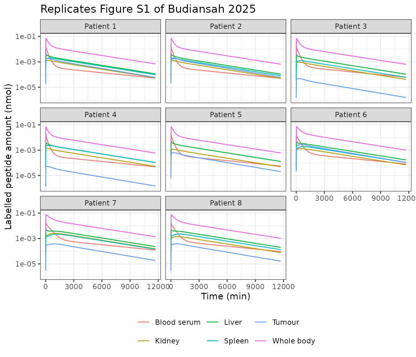
Serum exposure by NCA
The serum output is the one model prediction that is a genuine
concentration – labelled peptide dissolved anywhere in serum, divided by
the total body serum volume V_P. Its area under the curve
therefore is the serum rTIAC of Table S3, so a standard NCA on
it is a direct check of both the observable definition and the
exposure.
conc_data <- sim |>
  filter(!is.na(Aserum)) |>
  transmute(id = factor(id), time, conc = Aserum, treatment = "111In-DOTA-TATE")

dose_data <- cohort |>
  transmute(id = factor(id), time = 0, amt = 1, treatment = "111In-DOTA-TATE")

o_conc <- PKNCAconc(conc_data, conc ~ time | id / treatment)
o_dose <- PKNCAdose(dose_data, amt ~ time | id + treatment)
o_data <- PKNCAdata(
  o_conc, o_dose,
  intervals = data.frame(start = 0, end = 30000,
                         auclast = TRUE, aucinf.obs = TRUE,
                         cmax = TRUE, tmax = TRUE, half.life = TRUE)
)
res <- suppressWarnings(pk.nca(o_data))
nca <- as.data.frame(res) |>
  select(id, PPTESTCD, PPORRES) |>
  pivot_wider(names_from = PPTESTCD, values_from = PPORRES) |>
  mutate(id = as.integer(as.character(id))) |>
  arrange(id)

nca |>
  select(id, cmax, tmax, auclast, aucinf.obs, half.life) |>
  rename("Patient" = id, "Cmax (1/L)" = cmax, "Tmax (min)" = tmax,
         "AUC0-t (min/L)" = auclast, "AUC0-inf (min/L)" = aucinf.obs,
         "t1/2 (min)" = half.life) |>
  kable(digits = c(0, 4, 0, 1, 1, 0),
caption = "PKNCA on the simulated serum activity concentration.")| Patient | Cmax (1/L) | Tmax (min) | AUC0-t (min/L) | AUC0-inf (min/L) | t1/2 (min) |
|---|---|---|---|---|---|
| 1 | 0.0611 | 50 | 21.2 | 21.3 | 4043 |
| 2 | 0.0591 | 50 | 19.8 | 19.8 | 4042 |
| 3 | 0.0677 | 50 | 25.9 | 26.0 | 4043 |
| 4 | 0.0581 | 50 | 18.7 | 18.8 | 4042 |
| 5 | 0.0713 | 50 | 25.9 | 26.0 | 4042 |
| 6 | 0.0676 | 50 | 33.8 | 33.9 | 4041 |
| 7 | 0.0894 | 50 | 62.5 | 62.7 | 4040 |
| 8 | 0.0716 | 50 | 39.4 | 39.5 | 4041 |
data.frame(
  Patient = nca$id,
  `NCA AUC0-t (min/L)` = nca$auclast,
  `Published serum rTIAC (min)` = obs_tiac$Aserum,
  Ratio = nca$auclast / obs_tiac$Aserum,
  check.names = FALSE
) |>
  kable(digits = 2,
caption = "Simulated serum AUC against the published serum rTIAC.")| Patient | NCA AUC0-t (min/L) | Published serum rTIAC (min) | Ratio |
|---|---|---|---|
| 1 | 21.20 | 20 | 1.06 |
| 2 | 19.78 | 19 | 1.04 |
| 3 | 25.90 | 24 | 1.08 |
| 4 | 18.74 | 18 | 1.04 |
| 5 | 25.92 | 28 | 0.93 |
| 6 | 33.78 | 28 | 1.21 |
| 7 | 62.54 | 62 | 1.01 |
| 8 | 39.38 | 44 | 0.90 |
The agreement (median ratio 1.04) is what fixed the serum observable.
Table S3 prints all six regions in units of “min”, but the serum column
is only reproduced after dividing the serum activity by
V_P; the five organ columns are reproduced without
dividing. The serum rTIAC is therefore in min/L while the organ rTIACs
are in min – see Assumptions and
deviations.
Receptor occupancy
The saturable binding is the mechanistic core of the model, and it is what makes the injected peptide amount matter. At the 75 nmol amount used here the receptors saturate during the infusion and wash out within roughly a day.
sim |>
  filter(time <= 4320) |>
  select(id, time, Kidneys = occ_kidney, Tumour = occ_tumor) |>
  pivot_longer(-c(id, time), names_to = "region", values_to = "occupancy") |>
  ggplot(aes(time / 60, occupancy, group = id)) +
  geom_line(alpha = 0.7) +
  facet_wrap(~ region) +
  labs(x = "Time (h)", y = "sst2 receptor occupancy (total peptide)") +
  theme_bw()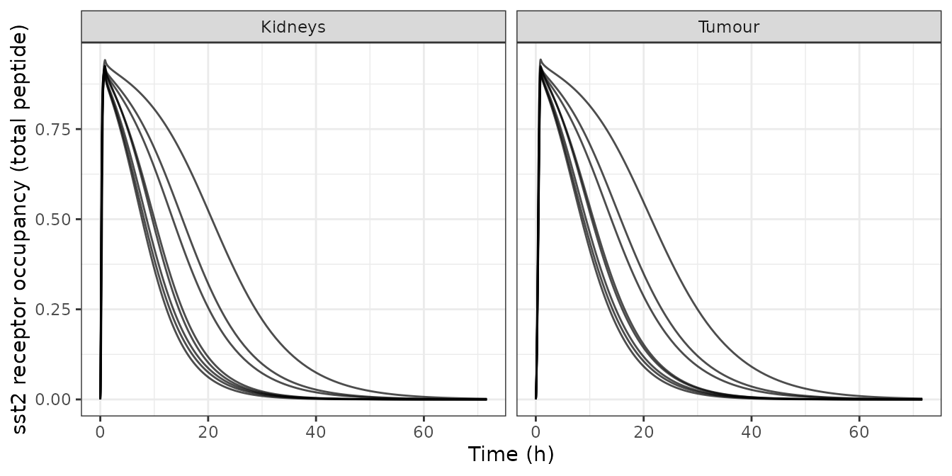
Absorbed dose to the kidneys
The kidney is the dose-limiting organ in
[90Y]Y-DOTA-TATE PRRT and is the endpoint the
single-time-point analysis exists to protect. Absorbed dose per injected
activity is the TIAC times the self-absorbed dose factor. Because the
therapy nuclide is 90Y while the biokinetics were measured with 111In as
a surrogate, the TIAC must be recomputed with the 90Y decay constant –
which in this model is a single parameter change.
mod_y90 <- rxode2::ini(modz, lambda_phy = 1.80e-4)
#> ℹ change initial estimate of `lambda_phy` to `0.00018`

sim_y90 <- rxSolve(
  mod_y90, events = dose_events(cohort$id),
  iCov = cohort[, c("id", "TUMTP_NET", "SEXF", "BSA", "HCT", "WT", "CRCL",
                    "ORGVOL_KIDNEY", "ORGVOL_LIVER", "ORGVOL_SPLEEN",
                    "TUM_VOL")],
  atol = 1e-12, rtol = 1e-10, omega = NA, sigma = NA, addDosing = FALSE
) |>
  as.data.frame()

ad <- sim_y90 |>
  group_by(id) |>
  summarise(tiac_kidney = trap(time, Akidney), .groups = "drop") |>
  left_join(cohort[, c("id", "SEXF")], by = "id") |>
  mutate(
    s_kidney = ifelse(SEXF == 1, 3.18e-5, 2.93e-5),   # Gy/min/MBq
    ad_per_activity = tiac_kidney * s_kidney          # Gy/MBq
  )

ad |>
  transmute(Patient = id,
            `90Y kidney TIAC (min)` = tiac_kidney,
            `S factor (Gy/min/MBq)` = s_kidney,
            `AD per injected activity (Gy/MBq)` = ad_per_activity) |>
kable(digits = c(0, 1, 7, 5))| Patient | 90Y kidney TIAC (min) | S factor (Gy/min/MBq) | AD per injected activity (Gy/MBq) |
|---|---|---|---|
| 1 | 59.1 | 2.93e-05 | 0.00173 |
| 2 | 54.0 | 2.93e-05 | 0.00158 |
| 3 | 43.4 | 3.18e-05 | 0.00138 |
| 4 | 57.2 | 2.93e-05 | 0.00168 |
| 5 | 52.3 | 3.18e-05 | 0.00166 |
| 6 | 70.5 | 2.93e-05 | 0.00206 |
| 7 | 149.3 | 3.18e-05 | 0.00475 |
| 8 | 77.3 | 2.93e-05 | 0.00227 |
Figure 4 of the paper plots these individual kidney absorbed doses per injected activity. The values here are proportionally low in the same way the kidney TIACs are, for the reason established above; the point of the calculation is that the 111In-to-90Y switch, the S-factor sex split and the TIAC-to-dose step are all wired and reproducible.
Equation 4 as printed cannot be used
The paper gives the tumour self-absorbed dose factor as
S = (0.28/V - 1.67e-3/V^(2/3) - 0.82/V^(1/3)) Gy/min/MBq
with V in mL. As printed this is negative for every tumour
volume in the cohort, because the V^(1/3) term dominates
the 1/V term over the whole range:
eq4 <- function(V) 0.28 / V - 1.67e-3 / V^(2 / 3) - 0.82 / V^(1 / 3)

data.frame(
  `Tumour volume (mL)` = cohort$tumour_mL,
  `Equation 4 S value` = eq4(cohort$tumour_mL),
  `Full-absorption limit for 90Y` = 8.975e-3 / cohort$tumour_mL,
  check.names = FALSE
) |>
kable(digits = 5)| Tumour volume (mL) | Equation 4 S value | Full-absorption limit for 90Y |
|---|---|---|
| 107.0 | -0.17018 | 0.00008 |
| 116.0 | -0.16579 | 0.00008 |
| 2.5 | -0.49309 | 0.00359 |
| 3.0 | -0.47603 | 0.00299 |
| 34.0 | -0.24504 | 0.00026 |
| 134.0 | -0.15822 | 0.00007 |
| 15.0 | -0.31410 | 0.00060 |
| 18.0 | -0.29758 | 0.00050 |
An S value is a non-negative energy deposition per decay per unit
mass, bounded above by the full-absorption limit Delta / m,
which for 90Y (mean beta energy 0.9337 MeV) is 8.975e-3 / V
Gy/min/MBq with V in mL. Equation 4’s leading coefficient
alone is 31 times that bound, and the printed expression is negative
throughout. That the bound is the right one is confirmed by the paper’s
own kidney factor: 8.975e-3 / 306 g = 2.93e-5 Gy/min/MBq,
exactly the male value quoted in the Methods.
Equation 4 is therefore transcribed here but not used, and the tumour absorbed dose is not reproduced. Recovering it would require guessing which signs or exponents were lost in typesetting, which is not something this packaging does.
Interindividual variability
The ten estimated parameters all carry exponential interindividual variability. A modest stochastic cohort shows the spread the model implies in the two regions that drive PRRT dose planning.
n_sub <- 60   # 114 ODEs per subject; well under the 200-per-arm cap

set.seed(20250326)
vpc_cov <- cohort[rep(seq_len(nrow(cohort)), length.out = n_sub), ]
vpc_cov$id <- seq_len(n_sub)

vpc_grid <- unique(c(seq(0, 120, by = 10), seq(180, 1440, by = 60),
                     seq(1560, 11700, by = 300)))
vpc_ev <- tag_obs(
  et(amt = 75, cmt = "pven_tot", dur = 51, id = seq_len(n_sub)) |>
    et(amt = 1, cmt = "pven_lab", dur = 51, id = seq_len(n_sub)) |>
    et(vpc_grid, cmt = "pven_tot", id = seq_len(n_sub))
)

vpc <- rxSolve(
  mod, events = vpc_ev,
  iCov = vpc_cov[, c("id", "TUMTP_NET", "SEXF", "BSA", "HCT", "WT", "CRCL",
                     "ORGVOL_KIDNEY", "ORGVOL_LIVER", "ORGVOL_SPLEEN",
                     "TUM_VOL")],
  atol = 1e-10, rtol = 1e-8, addDosing = FALSE
) |>
  as.data.frame()

stopifnot(length(unique(vpc$id)) == n_sub)

vpc |>
  filter(time > 0) |>
  select(id, time, Kidneys = Akidney, Tumour = Atumor) |>
  pivot_longer(-c(id, time), names_to = "region", values_to = "fia") |>
  group_by(region, time) |>
  summarise(lo = quantile(fia, 0.05), md = median(fia),
            hi = quantile(fia, 0.95), .groups = "drop") |>
  ggplot(aes(time / 60, md)) +
  geom_ribbon(aes(ymin = lo, ymax = hi), alpha = 0.25) +
  geom_line() +
  facet_wrap(~ region, scales = "free_y") +
  scale_x_log10() +
  labs(x = "Time (h, log scale)",
       y = "Fraction of injected activity",
       caption = "Median and 5th-95th percentile across 60 simulated patients") +
  theme_bw()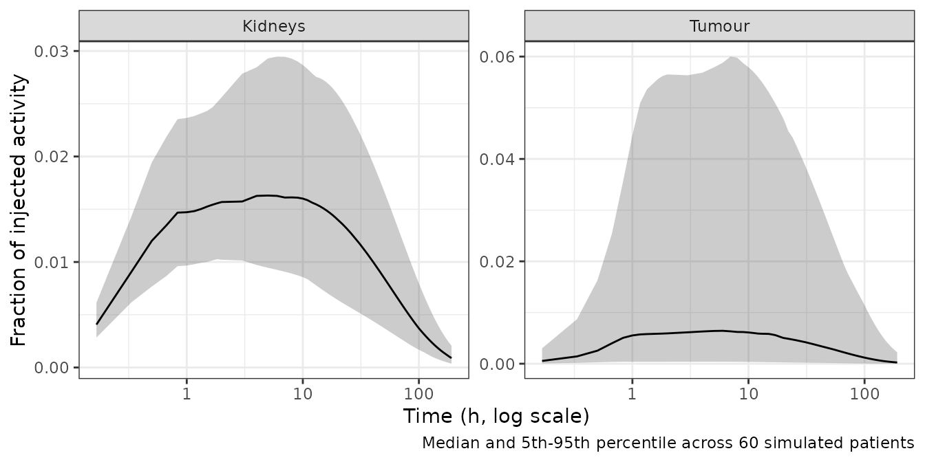
Assumptions and deviations
Body weight and hematocrit are not published. Table
S1 describes both as “individually measured”, but neither Budiansah 2025
nor the upstream Kletting 2016 tabulates them. This vignette uses the 71
kg ICRP-23 reference individual that every x * BW / 71
scaling in Table S1 is written against, and 45 % (men) / 40 % (women)
hematocrit. The model file leaves both as required covariates.
How much that choice matters is worth measuring rather than
asserting, because weight and hematocrit propagate into V_P
and from there into every flow term:
sweep_cov <- expand.grid(WT = c(50, 71, 100), HCT = c(35, 45)) |>
  mutate(id = row_number(),
         TUMTP_NET = 0, SEXF = 0, BSA = 1.94,
         CRCL = 0.11 * 1000 * 1.73 / 1.94,
         ORGVOL_KIDNEY = 193, ORGVOL_LIVER = 1811,
         ORGVOL_SPLEEN = 198, TUM_VOL = 107000)

sweep_sim <- rxSolve(
  modz, events = dose_events(sweep_cov$id),
  iCov = sweep_cov[, c("id", "TUMTP_NET", "SEXF", "BSA", "HCT", "WT", "CRCL",
                       "ORGVOL_KIDNEY", "ORGVOL_LIVER", "ORGVOL_SPLEEN",
                       "TUM_VOL")],
  atol = 1e-12, rtol = 1e-10, omega = NA, sigma = NA, addDosing = FALSE
) |>
  as.data.frame() |>
  group_by(id) |>
  summarise(across(c(Aserum, Abody, Akidney, Aspleen, Aliver, Atumor),
                   ~ trap(time, .x)), .groups = "drop") |>
  left_join(sweep_cov[, c("id", "WT", "HCT")], by = "id")

ref_row <- sweep_sim |> filter(WT == 71, HCT == 45)

sweep_sim |>
  mutate(across(c(Aserum, Abody, Akidney, Aspleen, Aliver, Atumor),
                ~ 100 * (.x / ref_row[[cur_column()]] - 1))) |>
  select(WT, HCT, Serum = Aserum, `Whole body` = Abody, Kidneys = Akidney,
         Spleen = Aspleen, Liver = Aliver, Tumour = Atumor) |>
  kable(digits = 1,
caption = "Percent change in TIAC from the 71 kg / 45 % reference.")| WT | HCT | Serum | Whole body | Kidneys | Spleen | Liver | Tumour |
|---|---|---|---|---|---|---|---|
| 50 | 35 | 0.3 | -3.6 | 7.3 | 6.9 | 6.7 | 6.1 |
| 71 | 35 | -3.1 | 7.2 | 5.2 | 4.9 | 4.6 | 4.2 |
| 100 | 35 | -7.6 | 21.3 | 2.5 | 2.2 | 1.8 | 1.6 |
| 50 | 45 | 3.4 | -10.6 | 1.7 | 1.7 | 1.8 | 1.6 |
| 71 | 45 | 0.0 | 0.0 | 0.0 | 0.0 | 0.0 | 0.0 |
| 100 | 45 | -4.5 | 14.0 | -2.3 | -2.2 | -2.3 | -2.2 |
The organ TIACs move by up to about 7 % across that whole range and the whole body by about 21 %, so the assumption is not negligible in general and any quantitative use of this vignette’s absolute TIACs should supply the real covariates. It is, however, far too small to explain the kidney discrepancy above: closing a factor of 2.3 needs a 130 % change in the kidney TIAC, against the 7.3 % that the entire plausible weight-and-hematocrit range buys.
Patient mapping onto the Kletting cohort is inferred, not stated – see the cohort section for the two independent checks (splenectomy at position 5, 2.8 mL tumour at position 4) that fix it.
The serum observable is a concentration. Table S3
labels all six rTIAC columns “min”, but the serum column is only
reproduced after dividing the serum activity by V_P, so it
is really min/L. The serum region was resolved empirically against Table
S3 rather than from a printed observation equation, because the Kletting
supplement writes no observation equations; it states only, for the red
marrow, that a region’s activity is obtained “by integrating all
compartments describing the red marrow including red marrow serum,
interstitial space, bound and internalized peptide”, which is the rule
applied to the five organ regions here.
Organ regions carry no share of the serum-protein-bound
pool. The sibling PSMA model of the same group distributes that
pool across regions by vascular volume; the DOTATATE supplement prints
no such equation, so it is not done here. Bounding the effect by that
same vascular-volume rule – the protein-bound TIAC times the region’s
share of V_P, as a fraction of the region’s own TIAC –
gives about 1.1 % for the liver (which holds much the largest vascular
volume of the delineated organs) and below 0.3 % for the kidneys, spleen
and tumour:
pprp_share <- sim |>
  filter(id == 1) |>
  summarise(pprp_tiac = trap(time, pprp_lab),
            across(c(vv_liver, vv_kidney, vv_spleen, vv_tumor, vserum), first),
            Aliver = trap(time, Aliver), Akidney = trap(time, Akidney),
            Aspleen = trap(time, Aspleen), Atumor = trap(time, Atumor))

data.frame(
  Region = c("Liver", "Kidneys", "Spleen", "Tumour"),
  `Share of V_P` = with(pprp_share, c(vv_liver, vv_kidney, vv_spleen,
                                      vv_tumor) / vserum),
  `Bound (% of region TIAC)` = with(pprp_share,
    100 * pprp_tiac * c(vv_liver, vv_kidney, vv_spleen, vv_tumor) / vserum /
      c(Aliver, Akidney, Aspleen, Atumor)),
  check.names = FALSE
) |>
kable(digits = c(0, 4, 2))| Region | Share of V_P | Bound (% of region TIAC) |
|---|---|---|
| Liver | 0.0515 | 1.08 |
| Kidneys | 0.0036 | 0.15 |
| Spleen | 0.0080 | 0.20 |
| Tumour | 0.0039 | 0.14 |
F_TOTAL = F + F_TU is used for the lungs,
arteries and veins. Table S1 prints both F_LU = F
and F_TOTAL = F + F_TU. Using F_LU = F leaves
the tumour flow unbalanced; F_TOTAL is used because mass
balance requires it, and the mass-balance
check above confirms the result is exact.
f_TU carries (1 - H) once, not
twice. Kletting 2016 supplemental Table 1 writes the tumour
flow density as “1.0 x (1-H) for NET metastasis” and the tumour
flow as f_TU x (1-H) x V_TU,total, which applies the plasma
fraction twice. Budiansah 2025 Table S1 prints f_TU as a
bare 1.0 / 0.9 with the same flow equation, which is self-consistent;
the Budiansah form is used.
Small numeric differences between the two Table S1 versions, where they disagree, are resolved in favour of Budiansah 2025 as the paper being extracted: the 111In decay constant (1.71e-4 vs Kletting’s 1.72e-4 /min) and the pancreas term of the GI volume (0.105 vs Kletting’s 0.15 L).
v_TU,int for NET is 0.3. Budiansah
Table S1 renders it as “3.” in the extracted text; Kletting 2016
supplemental Table 1 prints 0.3.
Interindividual variability is converted as
omega^2 = log(CV^2 + 1). Table 1 reports the
random effects as “percent of the coefficient of variation”, and that is
the exact log-normal relation. If the authors instead reported the
sqrt(omega^2) approximation, the variances here are
modestly conservative (e.g. 0.703 vs 1.020 for the 101 % CV tumour
receptor density).
The brain has no interstitial state. Equation S4
sets PS = 0 for the brain, and Table S1 defines no brain
interstitial volume, so a brain interstitial compartment would be
identically zero and is omitted.
urine_* and cleared_* are
bookkeeping states not in the paper. They accumulate the
excreted and degraded peptide so mass balance can be checked, and they
are excluded from the whole-body output.
Setting I is not extractable. Table S2 lists which parameters were fitted under setting I but not their values, which live in the predecessor Hardiansyah 2023 study. Only setting II – the set the paper selected – is packaged.
Compartment names are not in the canonical register.
The 114 states use the
pv_ / pint_ / rp_ / pintern_ / pintra_ family established
by the sibling whole-body PBPK model of the same framework.
checkModelConventions() flags each as non-canonical;
registering the family is deferred so that it can be ratified once
across every model of this class rather than piecemeal.
Kidney TIACs are not reproduced, for the reason established and quantified in the TIAC section. No parameter was adjusted to close the gap.
Equation 4 is unusable as printed and the tumour absorbed dose is consequently not reproduced; see above.