Elotuzumab with pomalidomide/dexamethasone (Ide 2022)
Source:vignettes/articles/Ide_2022_elotuzumab.Rmd
Ide_2022_elotuzumab.RmdModel and source
- Citation: Ide T, Osawa M, Sanghavi K, Vezina HE. Population pharmacokinetic and exposure-response analyses of elotuzumab plus pomalidomide and dexamethasone for relapsed and refractory multiple myeloma. Cancer Chemother Pharmacol. 2022;89(1):129-140.
- Article: https://doi.org/10.1007/s00280-021-04365-4 (open access; the model equations and final estimates are in the Supplementary Material: the full NONMEM control stream in the Supplementary Methods and the parameter estimates in Supplementary Table S2).
Elotuzumab is a humanized IgG1 monoclonal antibody against SLAMF7,
given with an immunomodulatory backbone in relapsed/refractory multiple
myeloma. Ide 2022 updates the earlier elotuzumab population PK model
(Gibiansky 2016; Ide 2020, available here as
Ide_2020_elotuzumab) with data from ELOQUENT-3, in which
elotuzumab was combined with pomalidomide/dexamethasone (Pd) and given
as 10 mg/kg weekly for two 28-day cycles followed by 20 mg/kg every 4
weeks.
The structure is unchanged from the earlier model: two compartments,
parallel linear and Michaelis-Menten elimination from the central
compartment, and second-order target-mediated elimination from the
peripheral compartment against a non-renewable target pool (initial
concentration RMAX):
Compared with Ide 2020, the update
- adds a pomalidomide/dexamethasone effect on linear CL (factor 0.811)
and on
KINT(factor 0.487), relative to the lenalidomide/dexamethasone (Ld) reference; - keeps the monotherapy contrast (CL x 1/0.825,
KINTx 1/9.78); - switches off the CL covariates of the earlier model (age, eGFR, LDH,
albumin, hepatic function, ECOG, sex, race and beta-2 microglobulin on
CL are all
0 FIXEDin the control stream), and keeps sex, Asian race and beta-2 microglobulin >= 3.5 mg/L on the central volume; - uses time-varying serum M-protein on
VMAX.
mod <- readModelDb("Ide_2022_elotuzumab")
mod_ui <- rxode2::rxode2(mod)
#> ℹ parameter labels from comments will be replaced by 'label()'
# zeroRe() warns that there are no sigma parameters: the residual SD is the
# model expression W, so there is nothing to zero on that side.
mod_typical <- suppressWarnings(rxode2::zeroRe(mod_ui))
Population
The model was fit to 8180 elotuzumab serum concentrations from 440 patients pooled from five trials (Ide 2022 Table 1): CA204-011 (elotuzumab monotherapy, high-risk smoldering myeloma), CA204-004 / ELOQUENT-2, CA204-005 and CA204-007 (with Ld), and CA204-125 / ELOQUENT-3 (with Pd). Median age was 66 years (37-88) and median body weight 75 kg (40-150); 41% were female and 13% Asian. Co-administration was monotherapy in 31 patients (7%), Ld in 349 (79%) and Pd in 60 (14%). Baseline serum M-protein had median 2.05 g/dL (0-7.7) and beta-2 microglobulin median 0.32 mg/dL (0.04-3.47).
The same information is available programmatically as
readModelDb("Ide_2022_elotuzumab") metadata
(population).
Source trace
Every value below is taken from Supplementary Table S2 (final estimates) of Ide 2022; the equations are from the Supplementary Methods NONMEM control stream.
| Model element | Value | Source |
|---|---|---|
lcl (CL_REF, L/day) |
log(0.0834) | Table S2, CLREF = exp(theta1) |
lvc (VC_REF, L) |
log(4.06) | Table S2, VCREF = exp(theta2) |
lq (Q_REF, L/day) |
log(0.512) | Table S2, QREF = exp(theta3) |
lvp (VP_REF, L) |
log(1.93) | Table S2, VPREF = exp(theta4) |
lrmax (ug/mL) |
log(849) | Table S2, RMAX = exp(theta5) |
lkint (mL/ug/day) |
log(0.216e-3) | Table S2, KINTREF = 0.216 x 10^-3 /day/(ug/mL); control stream
KINT = EXP(MU_6+ETA(6))/1000
|
lvmax (ug/mL/day) |
log(12.2) | Table S2, VMAXREF at MCPROT = 0 g/dL |
lkm (ug/mL) |
log(281) | Table S2, KM |
e_wt_cl, e_wt_vc, e_wt_q,
e_wt_vp
|
1.32, 0.345, 0.75 (fixed), 0.696 | Table S2, CLWT / VCWT / QWT / VPWT; reference 75 kg
(VWT = WT/75) |
e_mono_cl, e_mono_kint
|
log(0.825), log(9.78) | Table S2, CLMono / KINTMono, applied as (factor)^-Mono |
e_combo_pom_dex_cl,
e_combo_pom_dex_kint
|
log(0.811), log(0.487) | Table S2, CLPomDex / KINTPomDex |
e_sexf_vc, e_race_asian_vc
|
log(0.797), log(0.885) | Table S2, VCSEX / VCRACE |
e_b2m_ge35_vc |
log(1.11) | Table S2, VCB2MICG>0.35 (theta36); control stream
B2MICG.GE.0.35 mg/dL |
e_mcprot_vmax |
0.27 per g/dL | Table S2, VMAXMCPROT (theta23) |
| IIV CL / VC / Q / VP / RMAX / KINT / KM | 0.158 / 0.0361 / 0.454 / 0.133 / 0.189 / 1.69 / 0.385 | Table S2, omega2 |
| IIV VMAX | 0.0001 (fixed) | Table S2, footnote d |
etaruv (IIV on residual magnitude) |
0.183 | Table S2, omega2 epsilon |
sdL, sdH, sd50,
sdPhase12
|
2.46, 0.0976, 6.17 ug/mL, 0.843 | Table S2, SDL / SDH / SD50 / SDphase1,2 |
ODEs, target(0) = rmax
|
see above | control stream $DES, A_0(3)=RMAX
|
| Residual error |
W = (sdL - (sdL - sdH) Cc/(sd50 + Cc)) sdPhase12^(1 - STUDY_PHASE3) exp(etaruv),
Cc ~ lnorm(W)
|
control stream $ERROR:
W = (SDL-(SDL-SDH)*TY/(SD50+TY))*THETA(16)**STOTHER*EXP(ETA(9)),
Y = LOG(TY) + W*EPS(1), $SIGMA 1 FIXED
|
Covariate effects: checks against the paper’s statements
The Results state that CL at 50.6 kg (5th percentile) and 105 kg
(95th percentile) is about 41% lower and 55% higher than at the 75 kg
reference, and that Pd lowers linear CL by 19% and KINT by
51% relative to Ld. These are deterministic functions of the
typical-value parameters, so they are checked tightly.
ref_cov <- data.frame(
  WT = 75, SEXF = 0, RACE_ASIAN = 0, B2M = 3, MCPROT = 0,
  COMBO_LEN_DEX = 1, COMBO_POM_DEX = 0, STUDY_PHASE3 = 1
)
scenario <- function(label, ...) {
  out <- ref_cov
  changes <- list(...)
  for (nm in names(changes)) out[[nm]] <- changes[[nm]]
  out$scenario <- label
  out
}
scen <- dplyr::bind_rows(
  scenario("Reference (75 kg, Ld)"),
  scenario("WT 50.6 kg", WT = 50.6),
  scenario("WT 105 kg", WT = 105),
  scenario("Pd", COMBO_LEN_DEX = 0, COMBO_POM_DEX = 1),
  scenario("Monotherapy", COMBO_LEN_DEX = 0),
  scenario("Female", SEXF = 1),
  scenario("Asian", RACE_ASIAN = 1),
  scenario("B2M 3.5 mg/L", B2M = 3.5)
)
scen$id <- seq_len(nrow(scen))
ev_cov <- dplyr::bind_rows(
  dplyr::mutate(scen, time = 0, amt = 750, evid = 1L, cmt = "central"),
  dplyr::mutate(scen, time = 1, amt = 0, evid = 0L, cmt = "central")
) |>
  dplyr::arrange(id, time)

par_cov <- rxode2::rxSolve(mod_typical, events = ev_cov, keep = "scenario") |>
  as.data.frame() |>
  dplyr::distinct(scenario, cl, vc, kint)
#> ℹ omega/sigma items treated as zero: 'etalcl', 'etalvc', 'etalq', 'etalvp', 'etalrmax', 'etalkint', 'etalvmax', 'etalkm', 'etaruv'
#> Warning: multi-subject simulation without without 'omega'
ref_row <- par_cov[par_cov$scenario == "Reference (75 kg, Ld)", ]
par_cov <- par_cov |>
  dplyr::mutate(
    cl_ratio = cl / ref_row$cl,
    vc_ratio = vc / ref_row$vc,
    kint_ratio = kint / ref_row$kint
  )
par_cov |>
  dplyr::mutate(kint = kint * 1000) |>
  dplyr::rename(
    Scenario = scenario, `CL (L/day)` = cl, `VC (L)` = vc,
    `KINT (1e-3 mL/ug/day)` = kint, `CL ratio` = cl_ratio,
    `VC ratio` = vc_ratio, `KINT ratio` = kint_ratio
  ) |>
knitr::kable(digits = 4, caption = "Typical-value parameters relative to the reference patient.")| Scenario | CL (L/day) | VC (L) | KINT (1e-3 mL/ug/day) | CL ratio | VC ratio | KINT ratio |
|---|---|---|---|---|---|---|
| Reference (75 kg, Ld) | 0.0834 | 4.0600 | 0.2160 | 1.0000 | 1.0000 | 1.0000 |
| WT 50.6 kg | 0.0496 | 3.5446 | 0.2160 | 0.5948 | 0.8730 | 1.0000 |
| WT 105 kg | 0.1300 | 4.5597 | 0.2160 | 1.5592 | 1.1231 | 1.0000 |
| Pd | 0.0676 | 4.0600 | 0.1052 | 0.8110 | 1.0000 | 0.4870 |
| Monotherapy | 0.1011 | 4.0600 | 0.0221 | 1.2121 | 1.0000 | 0.1022 |
| Female | 0.0834 | 3.2358 | 0.2160 | 1.0000 | 0.7970 | 1.0000 |
| Asian | 0.0834 | 3.5931 | 0.2160 | 1.0000 | 0.8850 | 1.0000 |
| B2M 3.5 mg/L | 0.0834 | 4.5066 | 0.2160 | 1.0000 | 1.1100 | 1.0000 |
ratio <- function(s, col) par_cov[[col]][par_cov$scenario == s]
stopifnot(
  nrow(par_cov) == nrow(scen),
  abs(ratio("WT 50.6 kg", "cl_ratio") - (1 - 0.41)) < 0.01,
  abs(ratio("WT 105 kg", "cl_ratio") - (1 + 0.55)) < 0.01,
  abs(ratio("Pd", "cl_ratio") - (1 - 0.19)) < 0.005,
  abs(ratio("Pd", "kint_ratio") - (1 - 0.51)) < 0.005,
  abs(ratio("Monotherapy", "cl_ratio") - 1 / 0.825) < 1e-6,
  abs(ratio("Monotherapy", "kint_ratio") - 1 / 9.78) < 1e-6,
  abs(ratio("Female", "vc_ratio") - 0.797) < 1e-6,
  abs(ratio("Asian", "vc_ratio") - 0.885) < 1e-6,
  abs(ratio("B2M 3.5 mg/L", "vc_ratio") - 1.11) < 1e-6
)
Linear versus target-mediated elimination (Figure 1)
Figure 1 of Ide 2022 contrasts the constant linear clearance with the
Michaelis-Menten clearance from the central compartment, which falls as
the concentration rises. The Michaelis-Menten term
VMAX * central / (Cc + KM) is a clearance of
VMAX * VC / (Cc + KM).
ref_par <- ref_row
conc_grid <- 10^seq(0, 3, length.out = 200)
theta <- mod_ui$theta
clear <- dplyr::bind_rows(lapply(c(0, 2.05), function(mp) {
  vmax_i <- exp(theta[["lvmax"]]) * exp(theta[["e_mcprot_vmax"]] * mp)
  data.frame(
    conc = conc_grid,
    `Linear CL` = ref_par$cl,
    `Michaelis-Menten` = vmax_i * ref_par$vc / (conc_grid + exp(theta[["lkm"]])),
    MCPROT = paste(mp, "g/dL"),
    check.names = FALSE
  )
})) |>
  tidyr::pivot_longer(c(`Linear CL`, `Michaelis-Menten`), names_to = "pathway", values_to = "clearance")

ggplot(clear, aes(conc, clearance, colour = pathway, linetype = MCPROT)) +
  geom_line() +
  scale_x_log10("Elotuzumab concentration (ug/mL)") +
  scale_y_continuous("Clearance (L/day)") +
  theme_minimal()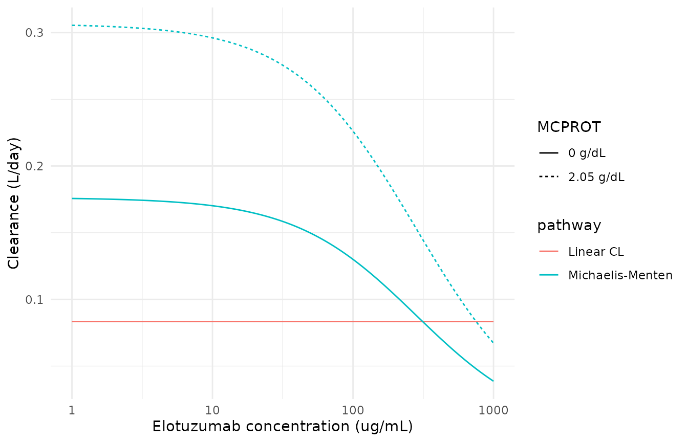
Replicates the idea of Figure 1 of Ide 2022: typical linear (nonspecific) clearance and Michaelis-Menten clearance from the central compartment versus elotuzumab concentration, at M-protein 0 and 2.05 g/dL (the dataset median).
Virtual cohort
The observed data are not public. The cohort below approximates Table 1 of Ide 2022: body weight normal (mean 75.6, SD 16.7 kg) redrawn until inside the observed 40-150 kg range; 41% female; 13% Asian; beta-2 microglobulin log-normal with median 3.2 mg/L (0.32 mg/dL); baseline M-protein gamma with the Table 1 mean 2.25 and SD 1.58 g/dL. M-protein is held at each subject’s baseline value for the whole simulation; see “Assumptions and deviations”. Two arms of 200 subjects share the same covariates:
- E-Ld: 10 mg/kg IV weekly for two 28-day cycles, then 10 mg/kg every 2 weeks (ELOQUENT-2 regimen);
- E-Pd: 10 mg/kg IV weekly for two 28-day cycles, then 20 mg/kg every 4 weeks (ELOQUENT-3 regimen).
rxode2::rxSetSeed(20220101)
set.seed(20220101)
n_per_arm <- 200L

draw_wt <- function(n) {
  out <- rnorm(n, 75.6, 16.7)
  bad <- out < 40 | out > 150
  while (any(bad)) {
    out[bad] <- rnorm(sum(bad), 75.6, 16.7)
    bad <- out < 40 | out > 150
  }
  out
}
mp_shape <- (2.25 / 1.58)^2
cohort <- data.frame(
  subj = seq_len(n_per_arm),
  WT = draw_wt(n_per_arm),
  SEXF = rbinom(n_per_arm, 1, 0.41),
  RACE_ASIAN = rbinom(n_per_arm, 1, 0.13),
  B2M = rlnorm(n_per_arm, log(3.2), 0.77),
  MCPROT = rgamma(n_per_arm, shape = mp_shape, scale = 2.25 / mp_shape)
)

infusion_days <- 2 / 24
end_day <- 392
regimen <- function(arm) {
  weekly <- seq(0, 49, by = 7)
  if (arm == "E-Ld") {
    maint <- seq(56, end_day - 14, by = 14)
    data.frame(time = c(weekly, maint), mg_per_kg = 10)
  } else {
    maint <- seq(56, end_day - 28, by = 28)
    data.frame(time = c(weekly, maint), mg_per_kg = c(rep(10, 8), rep(20, length(maint))))
  }
}

build_arm <- function(arm, id_offset) {
  doses <- regimen(arm)
  obs_times <- sort(unique(c(seq(0, end_day, by = 0.5), doses$time + infusion_days)))
  dplyr::bind_rows(lapply(seq_len(nrow(cohort)), function(i) {
    cov_i <- cohort[i, ]
    dose_rows <- data.frame(
      time = doses$time, amt = doses$mg_per_kg * cov_i$WT,
      dur = infusion_days, evid = 1L
    )
    obs_rows <- data.frame(time = obs_times, amt = 0, dur = 0, evid = 0L)
    dplyr::bind_rows(dose_rows, obs_rows) |>
      dplyr::mutate(
        id = id_offset + i, cmt = "central", treatment = arm,
        WT = cov_i$WT, SEXF = cov_i$SEXF, RACE_ASIAN = cov_i$RACE_ASIAN,
        B2M = cov_i$B2M, MCPROT = cov_i$MCPROT,
        COMBO_LEN_DEX = as.integer(arm == "E-Ld"),
        COMBO_POM_DEX = as.integer(arm == "E-Pd"),
        STUDY_PHASE3 = as.integer(arm == "E-Ld")
      )
  })) |>
    dplyr::arrange(id, time, dplyr::desc(evid))
}
events <- dplyr::bind_rows(build_arm("E-Ld", 0L), build_arm("E-Pd", 1000L))
stopifnot(all(table(unique(events[, c("id", "treatment")])$treatment) == n_per_arm))
Simulation
sim <- rxode2::rxSolve(mod_ui, events = events, keep = "treatment") |>
  as.data.frame()
stopifnot(all(is.finite(sim$Cc)), all(sim$Cc >= 0))
Concentration-time profiles (Figure 2)
prof <- sim |>
  dplyr::group_by(treatment, time) |>
  dplyr::summarise(
    median = median(Cc), p05 = quantile(Cc, 0.05), p95 = quantile(Cc, 0.95),
    .groups = "drop"
  )
ggplot(prof, aes(time / 7, median, colour = treatment, fill = treatment)) +
  geom_ribbon(aes(ymin = p05, ymax = p95), alpha = 0.2, colour = NA) +
  geom_line() +
  scale_x_continuous("Time since first dose (weeks)", breaks = seq(0, 56, by = 8)) +
  scale_y_continuous("Elotuzumab concentration (ug/mL)") +
  theme_minimal()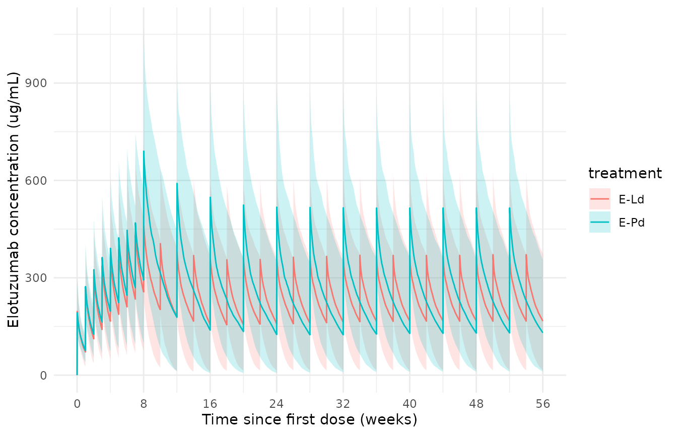
Replicates Figure 2 of Ide 2022: median (line) and 5th-95th percentile band of simulated elotuzumab concentrations for 10 mg/kg weekly (cycles 1-2) followed by 10 mg/kg Q2W with Ld, or 20 mg/kg Q4W with Pd.
PKNCA validation
Table 2 of Ide 2022 reports geometric means of the average, minimum
and maximum concentration over the first dosing interval (days 0-7) and
at steady state. For the first interval the minimum is the trough just
before the second dose on day 7 (PKNCA ctrough); the
interval minimum itself would be the pre-dose zero at time 0. The paper
states steady state is reached by about 16 weeks; the steady-state
interval used here is the maintenance interval starting on day 336 (week
48), which is 14 days for E-Ld and 28 days for E-Pd.
conc_df <- sim |>
  dplyr::filter(!is.na(Cc)) |>
  dplyr::select(id, time, Cc, treatment)
dose_df <- events |>
  dplyr::filter(evid == 1L) |>
  dplyr::select(id, time, amt, treatment)

conc_obj <- PKNCA::PKNCAconc(conc_df, Cc ~ time | treatment + id, concu = "ug/mL", timeu = "day")
dose_obj <- PKNCA::PKNCAdose(dose_df, amt ~ time | treatment + id, doseu = "mg")

intervals <- data.frame(
  treatment = c("E-Ld", "E-Pd", "E-Ld", "E-Pd"),
  start = c(0, 0, 336, 336),
  end = c(7, 7, 350, 364),
  cmax = TRUE, cav = TRUE,
  ctrough = c(TRUE, TRUE, FALSE, FALSE),
  cmin = c(FALSE, FALSE, TRUE, TRUE)
)
nca_res <- PKNCA::pk.nca(PKNCA::PKNCAdata(conc_obj, dose_obj, intervals = intervals))

nca_geo <- as.data.frame(nca_res$result) |>
  dplyr::filter(PPTESTCD %in% c("cmax", "cmin", "ctrough", "cav")) |>
  dplyr::mutate(
    interval = ifelse(start == 0, "First dose", "Steady state"),
    # Table 2 calls the first-interval trough Cmin1.
    PPTESTCD = ifelse(PPTESTCD == "ctrough", "cmin", PPTESTCD)
  ) |>
  dplyr::group_by(treatment, interval, PPTESTCD) |>
  dplyr::summarise(
    n = dplyr::n(),
    PPORRES = exp(mean(log(PPORRES))),
    .groups = "drop"
  )
stopifnot(all(nca_geo$n == n_per_arm), nrow(nca_geo) == 12L)
Comparison against published exposures
published <- data.frame(
  treatment = c("E-Ld", "E-Pd", "E-Ld", "E-Pd"),
  interval = c("First dose", "First dose", "Steady state", "Steady state"),
  cav = c(114, 113, 260, 266),
  cmin = c(63.4, 69.7, 179, 124),
  cmax = c(195, 185, 394, 543)
)
cmp <- nlmixr2lib::ncaComparisonTable(
  simulated = dplyr::select(nca_geo, -n),
  reference = published,
  by = c("treatment", "interval"),
  units = c(cav = "ug/mL", cmin = "ug/mL", cmax = "ug/mL")
)
knitr::kable(cmp, caption = "Geometric means: Ide 2022 Table 2 versus the simulated cohort.")| NCA parameter | treatment | interval | Reference | Simulated | % diff |
|---|---|---|---|---|---|
| Cmax (ug/mL) | E-Ld | First dose | 195 | 194 | -0.4% |
| Cmax (ug/mL) | E-Ld | Steady state | 394 | 349 | -11.4% |
| Cmax (ug/mL) | E-Pd | First dose | 185 | 195 | +5.6% |
| Cmax (ug/mL) | E-Pd | Steady state | 543 | 527 | -3.0% |
| Cmin (ug/mL) | E-Ld | First dose | 63.4 | 64.9 | +2.4% |
| Cmin (ug/mL) | E-Ld | Steady state | 179 | 126 | -29.8%* |
| Cmin (ug/mL) | E-Pd | First dose | 69.7 | 72.6 | +4.2% |
| Cmin (ug/mL) | E-Pd | Steady state | 124 | 92.5 | -25.4%* |
| Cavg (ug/mL) | E-Ld | First dose | 114 | 114 | -0.2% |
| Cavg (ug/mL) | E-Ld | Steady state | 260 | 209 | -19.4% |
| Cavg (ug/mL) | E-Pd | First dose | 113 | 118 | +4.4% |
| Cavg (ug/mL) | E-Pd | Steady state | 266 | 236 | -11.2% |
if (!is.null(attr(cmp, "footnote"))) cat(attr(cmp, "footnote"))
#> * differs from reference by more than ±20%.

geo <- function(trt, int, p) {
  nca_geo$PPORRES[nca_geo$treatment == trt & nca_geo$interval == int & nca_geo$PPTESTCD == p]
}
stopifnot(
  # First-dose exposure depends on the dose, VC and linear/MM clearance but
  # hardly on the M-protein trajectory, so it pins the structural model.
  abs(geo("E-Ld", "First dose", "cav") / 114 - 1) < 0.15,
  abs(geo("E-Pd", "First dose", "cav") / 113 - 1) < 0.15,
  abs(geo("E-Ld", "First dose", "cmin") / 63.4 - 1) < 0.15,
  abs(geo("E-Pd", "First dose", "cmin") / 69.7 - 1) < 0.15,
  # The Q4W regimen gives a higher peak and a lower trough than Q2W at steady
  # state (Table 2: +38% and -31%).
  geo("E-Pd", "Steady state", "cmax") / geo("E-Ld", "Steady state", "cmax") > 1.2,
  geo("E-Pd", "Steady state", "cmin") < geo("E-Ld", "Steady state", "cmin")
)
All three first-dose geometric means (Cavg1, Cmin1, Cmax1) are within
about 6% of Table 2 for both regimens, and the steady-state regimen
contrast (higher peak and lower trough with 20 mg/kg Q4W) is reproduced.
The steady-state values fall below the published geometric means, by
about 3-11% for Cmax, 11-19% for Cavg and 25-30% for Cmin. The trough is
the most sensitive to the Michaelis-Menten pathway, which is largest at
low concentrations. The shortfall is expected because the cohort holds
M-protein at its baseline value. In the trials M-protein fell during
treatment in most patients (Discussion of Ide 2022), which lowers
VMAX and raises steady-state exposure, and the paper
derived its exposures from each patient’s measured, linearly
interpolated M-protein.
Assumptions and deviations
-
M-protein held constant.
MCPROTis time-varying in the model and the paper interpolated each patient’s measurements. No M-protein trajectory is published, so the virtual cohort keeps each subject at a baseline value drawn to match Table 1. This is the main reason the simulated steady-state exposures are lower than Table 2. To simulate a responding patient, supplyMCPROTas a declining time series on the event rows. - Infusion duration. The paper models a zero-order infusion but does not state the infusion duration; 2 hours is assumed for all doses.
-
Backbone columns. The source control stream’s
LENDEXflag is 1 for every non-monotherapy study, including the Pd study, so it means “any immunomodulatory backbone”. The model uses two mutually exclusive indicators instead,COMBO_LEN_DEX(Ld) andCOMBO_POM_DEX(Pd), with monotherapy when both are 0; the monotherapy factors (CLMono, KINTMono) are applied as(factor)^-monoexactly as in Table S2. -
Residual error. The saturable log-scale residual
error is encoded as in the control stream, including the study
multiplier (
sdPhase12= 0.843 for the phase 1/2 studies, selected bySTUDY_PHASE3 = 0) and the inter-individual variability on the residual magnitude (etaruv). The control stream’s floorLTY = -2.5for non-positive predictions is not needed in simulation. -
Fixed-to-zero covariates. The control stream
carries twelve CL and VC covariate terms of the predecessor model as
0 FIXED(theta24-theta35). They contribute nothing and are listed in the model’scovariatesDataExcludedmetadata rather than in the model. -
Beta-2 microglobulin units. The dataset column is
in mg/dL with the threshold at 0.35 mg/dL; the model takes the canonical
B2Min mg/L with the equivalent 3.5 mg/L threshold. Table S2 labels the effect “VCB2MICG>0.35” while the control stream uses.GE.; the model follows the control stream (>=). - Exposure-response models not included. The paper’s exposure-response analyses are semi-parametric Cox proportional-hazards models (unspecified baseline hazard) of progression-free survival and grade 3+ adverse events on daily time-varying average concentration. Without a parametric baseline hazard they cannot be simulated, so only the population PK model is provided.